Power, Exponential, and Logistic Regression via Pseudoinverse

by Justin Skycak on January 03, 2022

Transforming nonlinear functions so that we can fit them using the pseudoinverse.

This post is a chapter in the book Introduction to Algorithms and Machine Learning: from Sorting to Strategic Agents. Suggested citation: Skycak, J. (2022). Power, Exponential, and Logistic Regression via Pseudoinverse. Introduction to Algorithms and Machine Learning: from Sorting to Strategic Agents. https://justinmath.com/power-exponential-and-logistic-regression-via-pseudoinverse/

Previously, we learned that we can use the pseudoinverse to fit any regression model that can be expressed as a linear combination of functions. Unfortunately, there are a handful of useful models that cannot be expressed as a linear combination of functions. Here, we will explore $3$ of these models in particular.

$\begin{align*} \textrm{Power regression: } y &= a \cdot x^b \\[5pt] \textrm{Exponential regression: } y &= a \cdot b^x \\[5pt] \textrm{Logistic regression: } y &= \dfrac{1}{1 + e^{-(ax+b)}} \end{align*}$

The techniques that we will learn for fitting these models will apply more generally to any model that can be transformed into a linear combination of functions (where the parameters are the coefficients in the linear combination).

Power and Exponential Regressions

Power and exponential regressions are familiar algebraic functions, so we will address them first. To transform a power or exponential regression into a linear combination of functions, we can transform the equation by taking the natural logarithm of both sides and applying the laws of logarithms to pull apart the expression on the right-hand side:

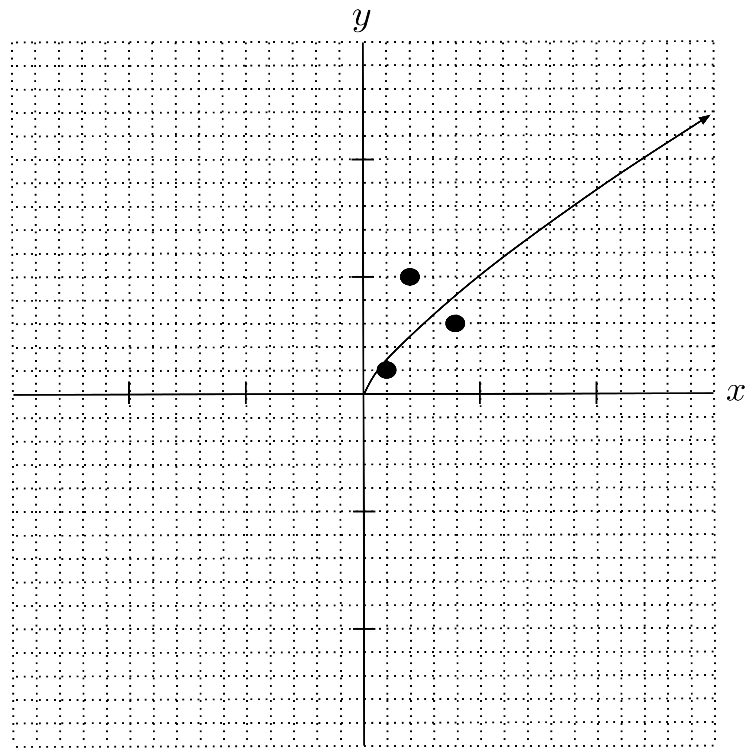
$\begin{align*} &\textrm{Power regression} \\ &\ln y = \ln \left( a \cdot x^b \right) \quad \to \quad \ln y = \ln a + b \ln x \\ \\ &\textrm{Exponential regression} \\ &\ln y = \ln \left( a \cdot b^x \right)\, \quad \to \quad \ln y = \ln a + (\ln b) \cdot x \end{align*}$

Let’s fit the power regression to the following data set.

$\begin{align*} \left[ (1,1), (2,5), (4,3) \right] \end{align*}$

As usual, we set up the system of equations, convert it into a matrix equation, and apply the pseudoinverse.

$\begin{align*} (x,y) \quad &\to \quad \ln y = (\ln a) \cdot 1 + b \cdot \ln x \\ \\ (1,1) \quad &\to \quad \ln 1 = (\ln a) \cdot 1 + b \cdot \ln 1 \quad \to \quad 0 = (\ln a) \cdot 1 + b \cdot 0 \\ (2,5) \quad &\to \quad \ln 5 = (\ln a) \cdot 1 + b \cdot \ln 2 \\ (4,3) \quad &\to \quad \ln 3 = (\ln a) \cdot 1 + b \cdot \ln 4 \end{align*}$

$\begin{align*} \begin{bmatrix} 0 \\ \ln 5 \\ \ln 3 \end{bmatrix} &= \begin{bmatrix} 1 & 0 \\ 1 & \ln 2 \\ 1 & \ln 4 \end{bmatrix} \begin{bmatrix} \ln a \\ b \end{bmatrix} \\[5pt] \begin{bmatrix} \ln a \\ b \end{bmatrix} &= \left( \begin{bmatrix} 1 & 1 & 1 \\ 0 & \ln 2 & \ln 4 \end{bmatrix} \begin{bmatrix} 1 & 0 \\ 1 & \ln 2 \\ 1 & \ln 4 \end{bmatrix} \right)^{-1} \begin{bmatrix} 1 & 1 & 1 \\ 0 & \ln 2 & \ln 4 \end{bmatrix} \begin{bmatrix} 0 \\ \ln 5 \\ \ln 3 \end{bmatrix} \\[5pt] &\approx \begin{bmatrix} 0.35 \\ 0.79 \end{bmatrix} \end{align*}$

So, we have the following model:

$\begin{align*} \ln y \approx 0.35 \cdot 1 + 0.79 \cdot \ln x \end{align*}$

By combining the logarithms and reversing the transformation that we originally applied to the power regression $y = a \cdot x^b,$ we can write the above model in power regression form:

$\begin{align*} \ln y &\approx 0.35 + 0.79 \cdot \ln x \\[5pt] \ln y &\approx \ln (e^{0.35}) + \ln x^{0.79} \\[5pt] \ln y &\approx \ln 1.42 + \ln x^{0.79} \\[5pt] \ln y &\approx \ln 1.42 \, x^{0.79} \\[5pt] y &\approx 1.42 \, x^{0.79} \end{align*}$

Danger: Unintentional Domain Constraints

Notice that the data set we used above was slightly different from the data set that we’ve used earlier in this chapter. We changed the $x$-coordinate $0$ to a $1$ in the first data point.

$\begin{align*} \textrm{Earlier: } [(\mathbf 0,1),(2,5),(4,3)] \\ \textrm{Now: } [(\mathbf 1,1),(2,5),(4,3)] \end{align*}$

The reason why we modified the data set is that the earlier data set exposes a limitation of the pseudoinverse method. We can’t fit our power regression model to the earlier data set, because the $x$-coordinate of $0$ causes a catastrophic issue in our transformed power regression equation.

To see what the issue is, let’s substitute the point $(0,1)$ into our transformed power regression equation and see what happens:

$\begin{align*} (x,y) \quad &\to \quad \ln y = (\ln a) \cdot 1 + b \cdot \ln x \\ (\mathbf 0,1) \quad &\to \quad \ln 1 = (\ln a) \cdot 1 + b \cdot \boxed{ \ln \mathbf 0 } \end{align*}$

The quantity $\ln 0$ is not defined, so $0$ is not a valid input for $x.$ By transforming the equation, we unintentionally imposed a constraint on the valid inputs $x.$

Danger: Suboptimal Fit

Unfortunately, this is not the only bad news. Even with our new data set, which does not contain any points with an $x$-value of $0,$ the pseudoinverse did not give us the most accurate fit of the power regression $y = ax^b.$ It gave us the most accurate fit of the transformed model $\ln y = (\ln a) \cdot 1 + b \cdot \ln x,$ but this is not the most accurate fit of the original power regression even though the two equations are mathematically equivalent.

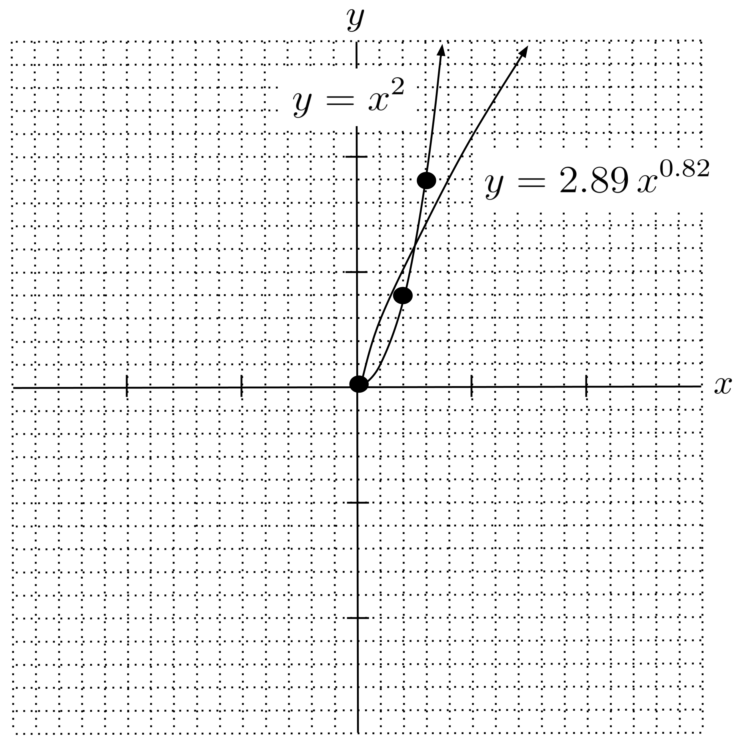
To understand this more clearly, let’s consider an extreme example. If we were to fit a power regression to the data set

$\begin{align*} \left[ (0.001, 0.01), (2,4), (3,9) \right] \end{align*}$

using the same method that we demonstrated above, then we would get the following model:

$\begin{align*} y \approx 2.89 \, x^{0.82} \end{align*}$

However, if we plot this curve along with the data, then it’s easy to see that this is not the most accurate model. It doesn’t even curve the right way! A hand-picked model as simple as $y = x^2$ would be vastly more accurate.

The reason the pseudoinverse method gave us an inaccurate model is that we transformed the model and data into a different space before we applied the pseudoinverse:

$\begin{align*} y = a \cdot x^b \quad \to \quad \ln y = (\ln a) \cdot 1 + b \cdot \ln x \end{align*}$

In the space that the data was transformed to, it turns out that the model $y \approx 2.89 \, x^{0.82}$ is more accurate than the model $y=x^2.$ To visualize this, we can plot these two models along with the data in the space of points $(\ln x, \ln y).$

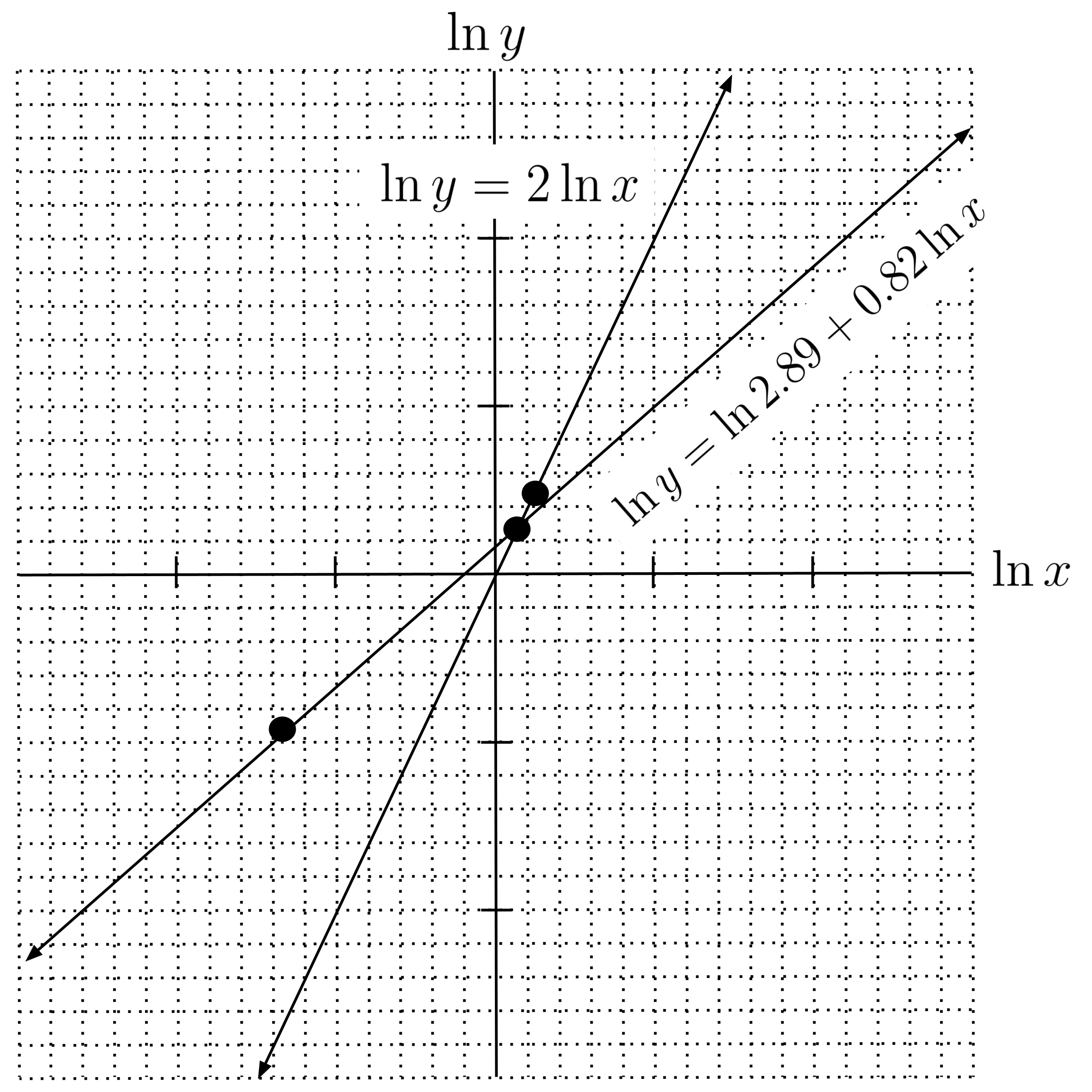
$\begin{align*} y = 2.89 \, x^{0.82} \quad &\to \quad \ln y = \ln 2.89 + 0.82 \ln x \\ y = x^2 \quad &\to \quad \ln y = 2 \ln x \\[5pt] [(0.001, 0.01), (2,4), (3,9)] \quad &\to \quad [(\ln 0.001, \ln 0.01), (\ln 2, \ln 4), (\ln 3,\ln 9)] \\ &\hspace{.9cm} \approx [(-6.91,-4.61), (0.69, 1.39), (1.10,2.20)] \end{align*}$

Indeed, $\ln y = \ln 2.89 + 0.82 \ln x$ is the most accurate model in the space of points $(\ln x, \ln y),$ but it is not the most accurate model in the space of points $(x,y).$

This is something to be cautious of whenever you transform a model into a space where the pseudoinverse can be applied – you should always check the function afterwards and verify that it is looks accurate “enough” for your purposes.

Logistic Regression

Soon, we will learn about other methods of fitting models that are robust to this sort of issue. But for now, let’s end by discussing the logistic function:

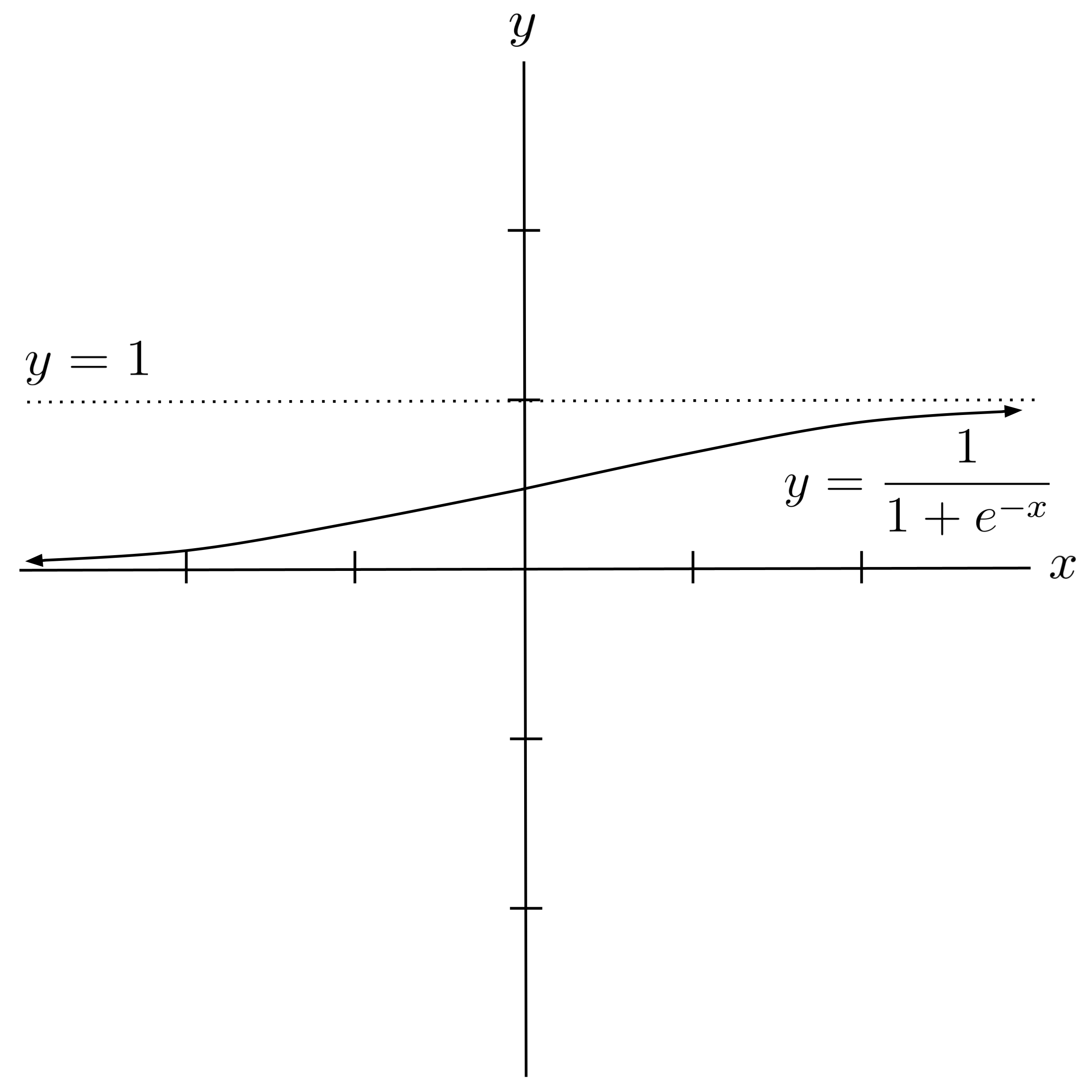
$\begin{align*} y &= \dfrac{1}{1 + e^{-(ax+b)}} \end{align*}$

The logistic function has a range of $0 < y < 1,$ and it is a common choice of model when the goal is to predict a bounded quantity. For example, probabilities are bounded between $0$ and $1,$ and rating scales (such as movie ratings) are often bounded between $1-5$ and $1-10.$

Let’s construct a real-life scenario in which to fit a logistic regression. Suppose that a food critic has rated sandwiches on a scale of $1-5$ as follows:

A roast beef sandwich with $1$ slice of roast beef was given a rating of $1$ out of $5.$
A roast beef sandwich with $2$ slices of roast beef was given a rating of $1$ out of $5.$
A roast beef sandwich with $3$ slices of roast beef was given a rating of $2$ out of $5.$

We will model the food critic’s rating as a function of the number of slices of roast beef. Our data set will consist of points $(x,y),$ where $x$ represents the number of slices of roast beef and $y$ represents the food critic’s rating.

$\begin{align*} [(1,1), (2,1), (3,2)] \end{align*}$

To model the rating, we can fit a logistic function and then round the output to the nearest whole number. Since the rating scale is between $1-5$ and we are going to round the output of the logistic function, we need to construct a logistic function with the range $0.5 < y < 5.5.$ We can do this as follows:

$\begin{align*} 0 &< \dfrac{1}{1+e^{-(ax+b)}} < 1 \\[5pt] 0 &< \dfrac{5}{1+e^{-(ax+b)}} < 5 \\[5pt] 0.5 &< \dfrac{5}{1+e^{-(ax+b)}} + 0.5 < 5.5 \end{align*}$

So, our goal is to fit the following model to the data set $[(1,1), (2,1), (3,2)].$

$\begin{align*} y = \dfrac{5}{1+e^{-(ax+b)}} + 0.5 \end{align*}$

In order to fit the model using the pseudoinverse, we need to transform it into a linear combination of functions. We do so by manipulating the equation to isolate the $ax+b{:}$

$\begin{align*} y &= \dfrac{5}{1+e^{-(ax+b)}} + 0.5 \\[5pt] y - 0.5 &= \dfrac{5}{1+e^{-(ax+b)}} \\[5pt] 1+e^{-(ax+b)} &= \dfrac{5}{y - 0.5} \\[5pt] e^{-(ax+b)} &= \dfrac{5}{y - 0.5} - 1 \\[5pt] -(ax+b) &= \ln \left( \dfrac{5}{y - 0.5} - 1 \right) \\[5pt] -\ln \left( \dfrac{5}{y - 0.5} - 1 \right) &= ax+b \end{align*}$

Now, we can proceed with the usual process of fitting our model using the pseudoinverse.

$\begin{align*} (x,y) \quad &\to \quad -\ln \left( \dfrac{5}{y - 0.5} - 1 \right) = a \cdot x+b \cdot 1 \\ \\ (1,1) \quad &\to \quad -\ln \left( \dfrac{5}{1 - 0.5} - 1 \right) = a \cdot 1 +b \cdot 1 \quad \to \quad - \ln 9 = a \cdot 1 + b \cdot 1 \\ (2,1) \quad &\to \quad -\ln \left( \dfrac{5}{1 - 0.5} - 1 \right) = a \cdot 2 +b \cdot 1 \quad \to \quad - \ln 9 = a \cdot 2 + b \cdot 1 \\ (3,2) \quad &\to \quad -\ln \left( \dfrac{5}{2 - 0.5} - 1 \right) = a \cdot 3 +b \cdot 1 \quad \to \quad - \ln (7/3) = a \cdot 3 + b \cdot 1 \end{align*}$

$\begin{align*} \begin{bmatrix} -\ln 9 \\ -\ln 9 \\ -\ln (7/3) \end{bmatrix} &= \begin{bmatrix} 1 & 1 \\ 2 & 1 \\ 3 & 1 \end{bmatrix} \begin{bmatrix} a \\ b \end{bmatrix} \\[5pt] \begin{bmatrix} a \\ b \end{bmatrix} &= \left( \begin{bmatrix} 1 & 2 & 3 \\ 1 & 1 & 1 \end{bmatrix} \begin{bmatrix} 1 & 1 \\ 2 & 1 \\ 3 & 1 \end{bmatrix} \right)^{-1} \begin{bmatrix} 1 & 2 & 3 \\ 1 & 1 & 1 \end{bmatrix} \begin{bmatrix} -\ln 9 \\ -\ln 9 \\ -\ln (7/3) \end{bmatrix} \\[5pt] &\approx \begin{bmatrix} 0.67 \\ -3.10 \end{bmatrix} \end{align*}$

So, we have the following model:

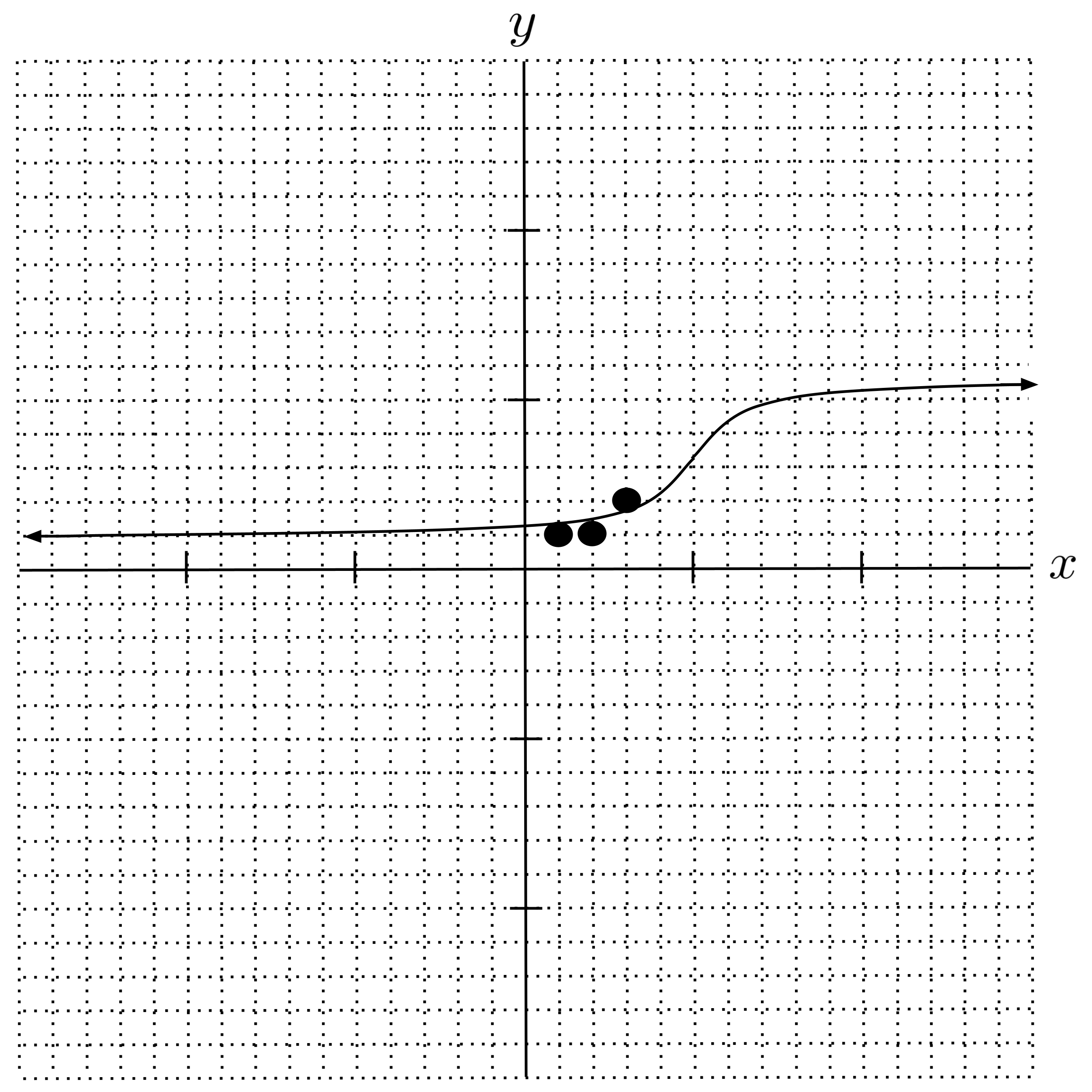
$\begin{align*} y \approx \dfrac{5}{1+e^{-(0.67x-3.10)}} + 0.5 \end{align*}$

Since we had to transform the model into a space where the pseudoinverse can be applied, we need to check the function and verify that it looks accurate enough for our purposes. Here, our regression curve looks fairly accurate, so we will proceed to analyze it.

Now that we have a regression curve, we can use it to make predictions about the data. For example, what rating would we expect the critic to give a sandwich with $6$ slices of roast beef? To answer this question, we just plug $x=6$ into our model:

$\begin{align*} y(6) &\approx \dfrac{5}{1+e^{-((0.67)(6) - 3.10)}} + 0.5 \\ &\approx 4.08 \end{align*}$

Our result of $4.08$ rounds to $4.$ So, according to our model, we predict that the critic would give a rating of $4$ to a sandwich that had $6$ slices of roast beef.

Exercises

Use the pseudoinverse method to fit each model to the given data set. Check your answer each time by sketching the resulting model on a graph containing the data points and verifying that it visually appears to capture the trend of the data.

Fit a power regression $y = a \cdot x^b$ to $[(1,0.2), (2,0.3), (3,0.5)].$
Fit an exponential regression $y = a \cdot b^x$ to $[(1,0.2), (2,0.3), (3,0.5)].$
Fit a logistic regression $y = \dfrac{1}{1+e^{-(ax+b)}}$ to $[(1,0.2), (2,0.3), (3,0.5)].$
Construct a logistic regression whose range is $0.5 < y < 10.5$ and fit it to $[(1,2), (2,3), (3,5)].$