Overfitting, Underfitting, Cross-Validation, and the Bias-Variance Tradeoff

by Justin Skycak on January 04, 2022

Just because model appears to match closely with points in the data set, does not necessarily mean it is a good model.

This post is a chapter in the book Introduction to Algorithms and Machine Learning: from Sorting to Strategic Agents. Suggested citation: Skycak, J. (2022). Overfitting, Underfitting, Cross-Validation, and the Bias-Variance Tradeoff. Introduction to Algorithms and Machine Learning: from Sorting to Strategic Agents. https://justinmath.com/overfitting-underfitting-cross-validation-and-the-bias-variance-tradeoff/

We have previously described a model as “accurate” when it appears to match closely with points in the data set. However, there are issues with this definition that we will need to remedy. In this chapter, we will expose these issues and develop a more nuanced understanding of model accuracy by way of a concrete example.

Overfitting and Underfitting

Consider the following data set of points $(x,y),$ where $x$ is the number of seconds that have elapsed since a rocket has launched and $y$ is the height (in meters) of the rocket above the ground. The data is noisy, meaning that there is some random error in the measurements.

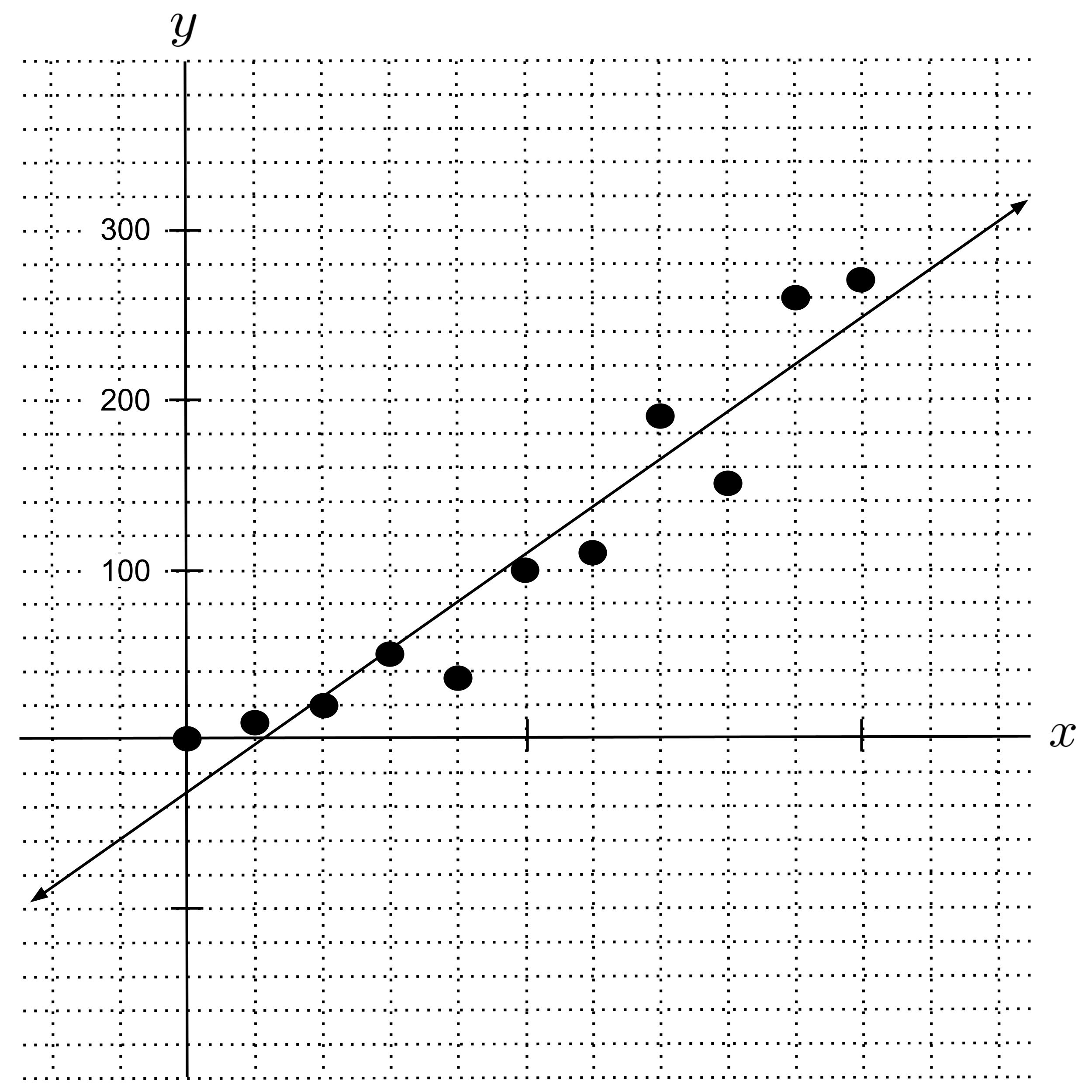
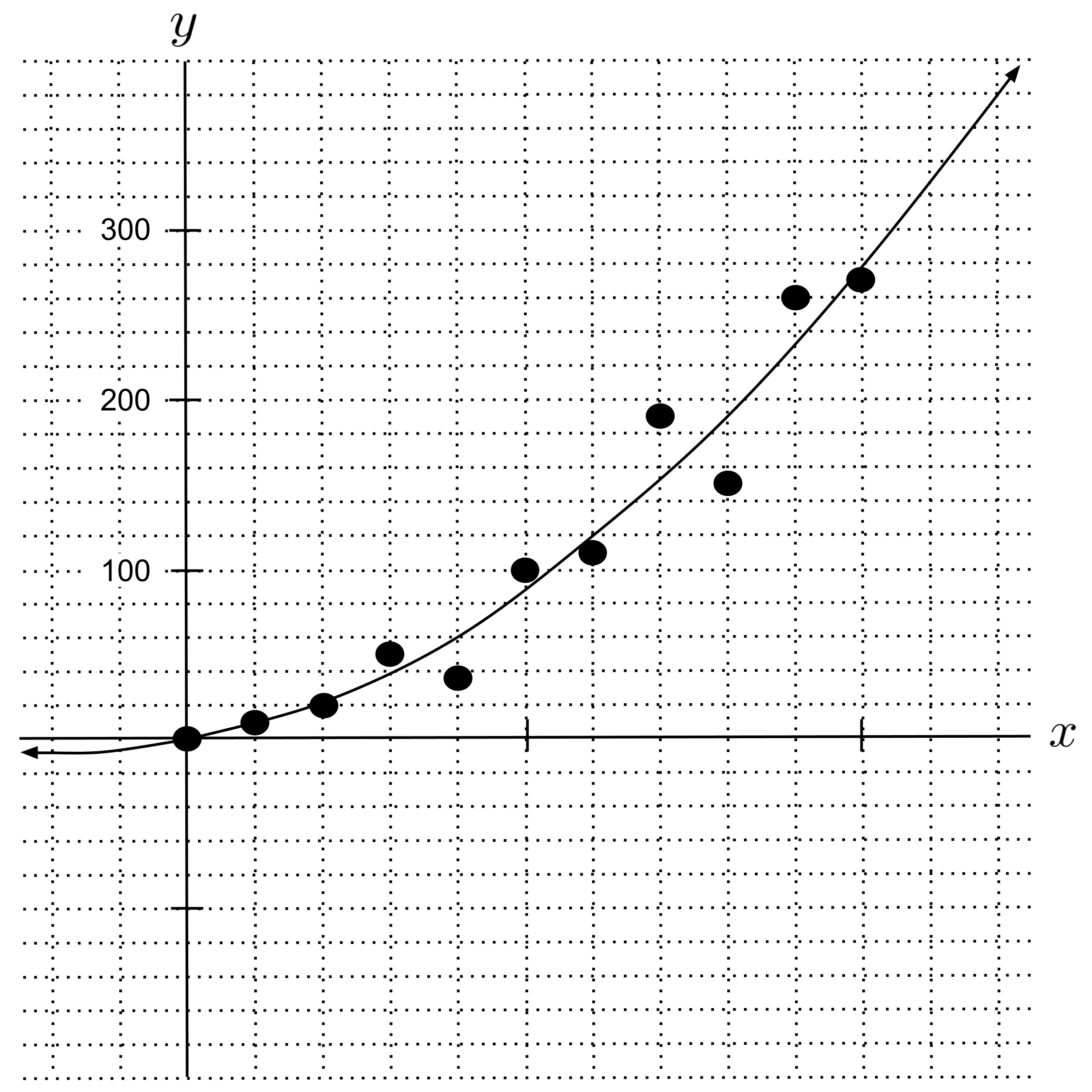
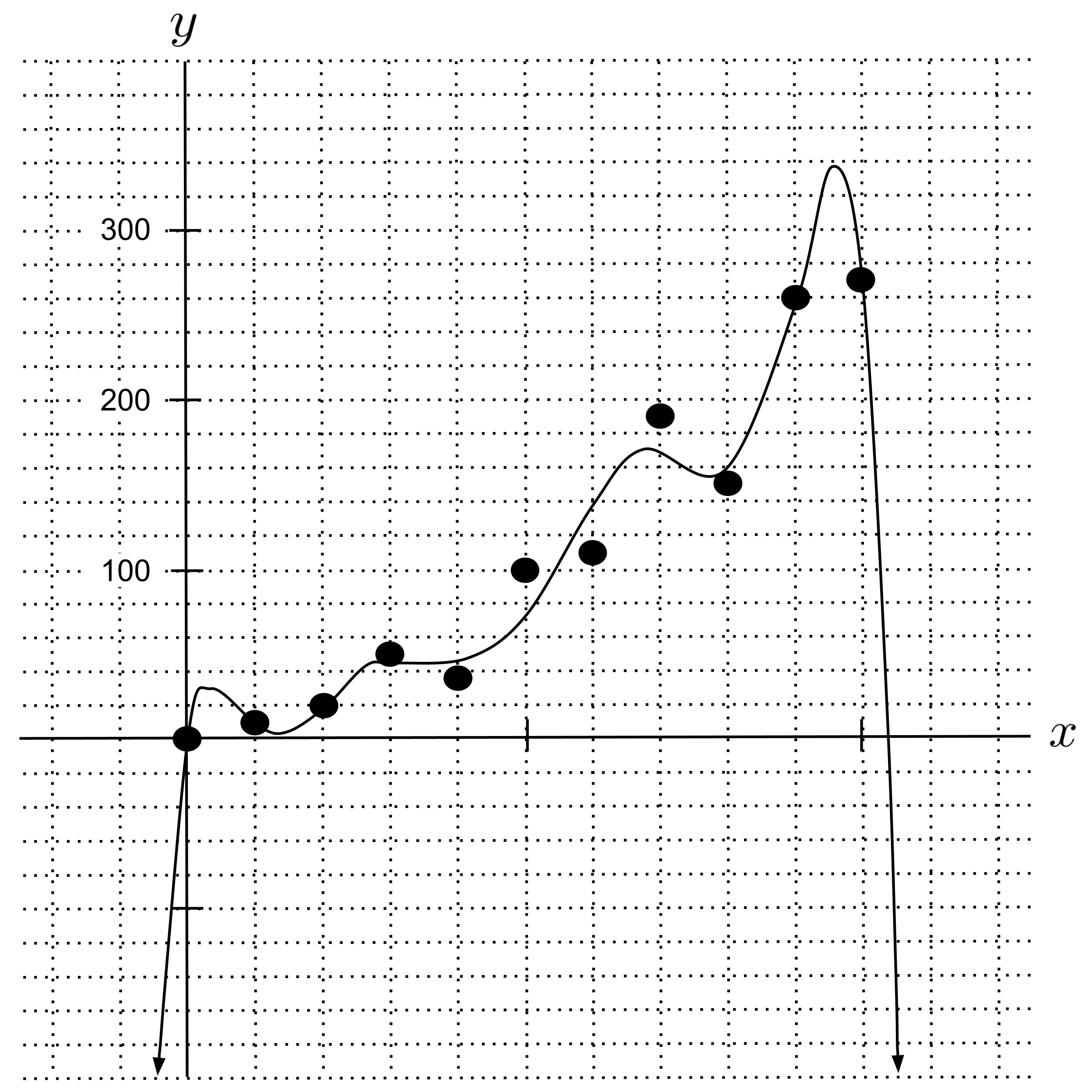
$\begin{align*} [&(0,0),(1,10),(2,20),(3,50),(4,35),(5,100), \\ &(6,110),(7,190),(8,150),(9,260),(10,270)] \end{align*}$

If we use the pseudoinverse to fit linear, quadratic, and $8$th degree polynomial regressions, we get the following results. (You should do this yourself and verify that you get the same results.)

$\begin{align*} \textrm{Linear: } & y = 28.14x-32.05 \end{align*}$

$\begin{align*} \textrm{Quadratic: } & y = 2.05x^2+7.68x-1.36 \end{align*}$

$\begin{align*} 8\textrm{th degree: } & y = -0.00778x^{8}+0.296666x^{7}-4.575859x^{6} \\ &\phantom{y =} +36.618048x^{5} -162.04318x^{4}+390.1833x^{3}\\ &\phantom{y=}-462.14466x^{2}+212.239681x-0.087308 \end{align*}$

Note that we used more decimal places in the $8$th degree polynomial regressor because it is very sensitive to rounding. (If you round the coefficients to $2$ decimal places and plot the result, it will look wildly different.)

As we can see from the graph, the $8$th degree polynomial regressor matches closest with the points in the data set. So, if we define “accuracy” as simply matching with points in the data set, then we’d say the $8$th degree polynomial is the most accurate.

However, this doesn’t pass the sniff test. In order to match up with the points in the data set so well, the $8$th degree polynomial has to curve and contort itself in unrealistic ways between data points.

For example, between the last two points in the data set, the $8$th degree polynomial rises up and falls down sharply. Did the rocket really rise up $100$ meters and fall down $100$ meters between the $9$th and $10$th seconds? Probably not.
Likewise, the $8$th degree polynomial continues dropping sharply after the $10$th second and hits the $x$-axis shortly after. Is the rocket really plummeting to the ground? Based on the actual data points, it seems unlikely.

So, we can’t place much trust in the $8$th degree polynomial’s predictions. The $8$th degree polynomial thinks the relationship between $x$ and $y$ is more complicated than it actually is. When this happens, we say that the model overfits the data.

On the other hand, the linear regression does not capture the fact that the data is curving upwards. It thinks the relationship between $x$ and $y$ is less complicated than it actually is. When this happens, we say that the model underfits the data.

Based on the graph, the quadratic regressor looks the most accurate. It captures the fact that the data is curving upwards, but it does not contort itself in unrealistic ways between data points, and it does not predict that the rocket is going to fall straight down to the ground immediately after the $10$th second. The quadratic regressor neither overfits nor underfits. So, we can place more trust in its predictions.

The Need for Cross Validation

The discussion above suggests that our definition of accuracy should be based on how well a model predicts things, not how well it matches up with the data set. So, we have a new definition of what it means for a model to be accurate:

Old (bad) definition: The closer a model matches up with points in the data set, the more accurate it is.
New (good) definition: The better a model predicts data points that it hasn't seen (i.e. were not used during the model fitting procedure), the more accurate it is.

But how can we measure how well a model predicts data points that it hasn’t seen, if we are fitting it on the entire data set? The answer is surprisingly simple: when measuring the accuracy of a model, don’t fit the model on the entire data set. Instead, carry out the following procedure, known as leave-one-out cross validation:

Remove a point from the data set.
Fit the model to all points in the data set except the point that we removed.
Check how accurately the model would have predicted the point that we left out.
Place the point back in the data set.
Repeat steps $1-4$ for every point in the data set and add up how much each prediction was "off" by. This is called the cross-validation error.
The model with the lowest cross-validation error is the most accurate, i.e. it does the best job of predicting real data points that it has not seen before.

The phrase leave-one-out refers to when we remove a point from the data set. The phrase cross validation refers to when we have the model predict the point we removed: we’re validating that the model still does a good job of predicting points that it hasn’t already been fitted on. The word cross indicates that during our validation, we’re asking the model to “cross over” from points it has seen, to points it has not seen.

Example: Cross Validation

Let’s demonstrate the leave-one-out cross validation procedure by computing the cross-validation error for linear, quadratic, and $8$th degree polynomial regression models on our rocket launch data set. We should find that the quadratic regression has the lowest error, the linear regression has slightly higher error, and the $8$th degree polynomial has significantly higher error.

The table below shows some of the intermediate steps for computing the cross-validation error for linear regression. In each row of the table, we remove a point from the data set, fit a linear regression model to the remaining data, and then get the predicted $y$-value by plugging the $x$-coordinate of the removed point into the model.

$\begin{align*} \begin{matrix} \begin{matrix}\textrm{Removed}\\ \textrm{Point}\end{matrix} & \textrm{Remaining Data} & \textrm{Model} & \begin{matrix}\textrm{Predicted} \\ \textrm{Y-Value}\end{matrix} \\ \hline \\ (0,0) & {\tiny \begin{bmatrix} \phantom{(0,0),} & (1,10), & (2,20), \\ (3,50), & (4,35), & (5,100), \\ (6,110), & (7,190), & (8,150), \\ (9,260), & (10,270) \end{bmatrix}} & y=30.27x-47.0 & -47.0 \\[15pt] (1,10) & {\tiny \begin{bmatrix} (0,0) & \phantom{(1,10),} & (2,20), \\ (3,50), & (4,35), & (5,100), \\ (6,110), & (7,190), & (8,150), \\ (9,260), & (10,270) \end{bmatrix}} & y=28.8x-37.01 & -8.21 \\[15pt] (2,20) & {\tiny \begin{bmatrix} (0,0) & (1,10), & \phantom{(2,20),} \\ (3,50), & (4,35), & (5,100), \\ (6,110), & (7,190), & (8,150), \\ (9,260), & (10,270) \end{bmatrix}} & y=28.0x-30.88 & 25.12 \\[15pt] \vdots & \vdots & \vdots & \vdots \\[15pt] (10,270) & {\tiny \begin{bmatrix} (0,0) & (1,10), & (2,20), \\ (3,50), & (4,35), & (5,100), \\ (6,110), & (7,190), & (8,150), \\ (9,260), & \phantom{(10,270)} \end{bmatrix}} & y=26.76x-27.91 & 239.69 \\[15pt] \end{matrix} \end{align*}$

Once we have all the predicted points, we can compare them to the removed points and compute the cross-validation error. For each row in the table, we compute the square of the difference between the predicted $y$-value and the actual $y$-value in the removed point.

$\begin{align*} \begin{matrix} (x_\textrm{actual}, y_\textrm{actual}) & y_\textrm{predicted} & (y_\textrm{predicted} - y_\textrm{actual})^2 \\ \hline \\ (0,0) & -47.0 & (-47.0 - 0)^2 \\[3pt] (1,10) & -8.21 & (-8.21 - 10)^2 \\[3pt] (2,20) & 25.12 & (25.12 - 20)^2 \\[3pt] \vdots & \vdots & \vdots \\[3pt] (10,270) & 239.69 & (239.69 - 270)^2 \\[3pt] \end{matrix} \end{align*}$

Note that although it might feel more natural to take the absolute value instead of the square when computing the total error, it’s conventional to work with squared distances in machine learning and statistics because squaring has more desirable mathematical properties. For example, squaring is differentiable everywhere, whereas absolute value is not (the graph of the absolute value function is not differentiable at $0$).

Finally, we sum up all the individual squared errors to get the total cross-validation error. This sum of squared errors is also known as the cross-validated RSS (residual sum of squares).

$\begin{align*} (-47.0 - 0)^2 + (-8.21 - 10)^2 + (25.12 - 20)^2 + \ldots + (239.69 - 270)^2 \end{align*}$

If we compute the cross-validation error for the linear, quadratic, and $8$th degree polynomial regressors separately, then we get the following results (rounded to the nearest integer). Note that these results were generated via code, and there was no intermediate rounding like was done while working out the example above. You should try to calculate these cross-validation errors on your own and verify that your numbers match up.

$\begin{align*} \begin{matrix} \textrm{Model} & \textrm{Cross-Validation Error} \\ \hline \\[-8pt] \textrm{Linear} & 13 \, 143 \\ \textrm{Quadratic} & 8\,033 \\ 8\textrm{th Degree} & 7\,615\,290 \end{matrix} \end{align*}$

If you need to debug anything by hand and round intermediate results, remember to keep many decimal places in the coefficients of the $8$th degree polynomial regressor. (If you use too few decimal places, then the regressor will give wildly different results.)

The results are just as we expected:

The quadratic regressor has the lowest cross-validation error, which means it is the most accurate model to use for this data set.
The linear regressor has sightly higher cross-validation error because it slightly underfits the data (it doesn't capture the fact that the data is curving upwards).
The $8$th degree polynomial has massively higher cross-validation error because it massively overfits the data (it contorts itself and overcomplicates things so much that it thinks the rocket is plummeting to the ground).

Bias-Variance Tradeoff

Finally, let’s build more intuition about why these results came out as they did. It turns out that the total cross-validation error in our model is the sum of two different types of error:

$\begin{align*} \begin{pmatrix}\textrm{total cross-} \\ \textrm{validation error}\end{pmatrix} &= \begin{pmatrix}\textrm{error due}\\ \textrm{to bias}\end{pmatrix} + \begin{pmatrix}\textrm{error due}\\ \textrm{to variance}\end{pmatrix} \end{align*}$

Loosely speaking, error due to bias occurs if a model assumes too much about the relationship being modeled. In our example, the linear regressor had high error due to bias because it assumed that the relationship was a straight line (whereas the data was actually curving upwards a bit). The error due to bias comes from a model’s inability to pass through all the points that are being used to fit it. A model with high bias is too rigid to capture some trends in the data, and therefore underfits the data.

On the other hand, error due to variance occurs if a model changes drastically when fit to a different sample of data points from the same data set. In our example, the $8$th degree polynomial regressor had high error due to variance. To see this, you should plot all the different $8$th degree regressors that you came up with during your leave-one-out cross validation and observe that the graphs look quite different from one another. This is bad because a model is supposed to pick up on the true relationship underlying some data, and if the model changes its mind significantly when it’s shown different samples of data from the same data set, then we can’t trust it! A model with high variance is so flexible that it reads too much into the relationship between points in the data set and contorts itself in weird ways.

To build further intuition for bias and variance, it can help to anthropomorphize a bit:

A high-bias model is dumb: it can't comprehend the complexity of the relationship in the data.
A high-variance model is paranoid: it thinks it's seeing all sorts of complicated relationships that just aren't there.

Ideally, we would like to minimize error due to bias and error due to variance. However, bias and variance are two sides of the same coin: when one decreases, the other increases. By minimizing one, we maximize the other. In particular:

By making the model less rigid (i.e. decreasing bias), we make the model more flexible (i.e. increase variance).
By making the model less flexible (i.e. decreasing variance), we make the model more rigid (i.e. increase bias).

This is known as the the bias-variance tradeoff, and it means that we cannot simply minimize bias and variance independently. This is why cross-validation is so useful: it allows us to compute and thereby minimize the sum of error due to bias and error due to variance, so that we may find the ideal tradeoff between bias and variance.

K-Fold Cross Validation

In closing, note that although leave-one-out cross validation can take a long time to run on large data sets, a similar procedure called $k$-fold cross validation can be used instead. Instead of removing one point at a time, we shuffle the data set, break it up into $k$ parts (with each part containing roughly the same number of points), and then remove one of the parts each time. Each time, we predict the points in the part that we left out, and then we add up all the squared errors. We usually choose $k$ to be a small number (such as $k = 5$) so that the cross validation procedure runs fairly quickly.

Exercise

Work out the computations that were outlined in the examples above. Fit and compute leave-one-out cross validation error for linear, quadratic, and $8$th degree polynomials and verify that your results match up with the examples.