Regressing a Linear Combination of Nonlinear Functions via Pseudoinverse

by Justin Skycak on January 02, 2022

Exploring the most general class of functions that can be fit using the pseudoinverse.

This post is a chapter in the book Introduction to Algorithms and Machine Learning: from Sorting to Strategic Agents. Suggested citation: Skycak, J. (2022). Regressing a Linear Combination of Nonlinear Functions via Pseudoinverse. Introduction to Algorithms and Machine Learning: from Sorting to Strategic Agents. https://justinmath.com/regressing-a-linear-combination-of-nonlinear-functions-via-pseudoinverse/

Previously, we learned how to use the pseudoinverse to fit linear and polynomial models to data sets consisting of one or more input variables. However, the pseudoinverse is even more general than that.

Worked Example

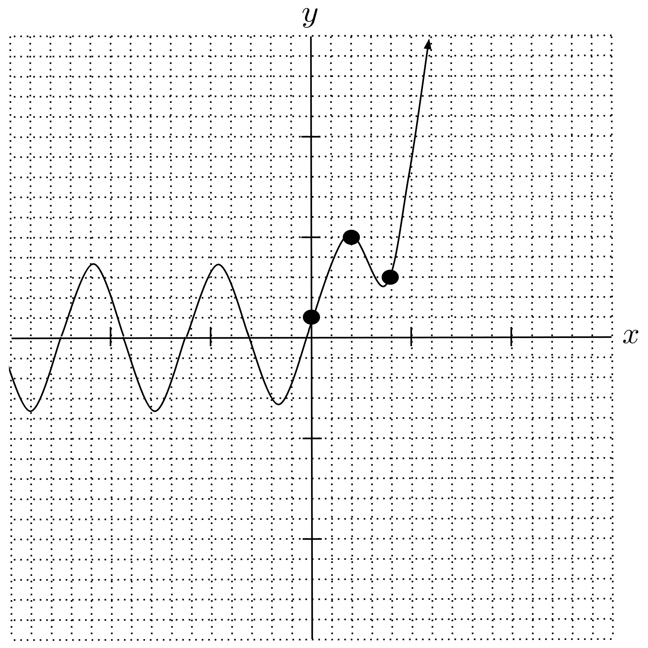
For example, let’s fit the model

$\begin{align*} y = a \sin x + b \cdot 2^x \end{align*}$

to the following data set:

$\begin{align*} \left[ (0,1), (2,5), (4,3) \right] \end{align*}$

Although the model is more complicated, the procedure for fitting it is exactly the same. First, we set up our system:

$\begin{align*} (x,y) \quad &\to \quad y = a \cdot \sin x + b \cdot 2^x \\ \\ (0,1) \quad &\to \quad 1 = a \cdot \sin 0 + b \cdot 2^0 \\ (2,5) \quad &\to \quad 5 = a \cdot \sin 2 + b \cdot 2^2 \\ (4,3) \quad &\to \quad 3 = a \cdot \sin 4 + b \cdot 2^4 \end{align*}$

Then we convert to a matrix equation and multiply both sides by the transpose of the coefficient matrix.

$\begin{align*} \begin{bmatrix} 1 \\ 5 \\ 3 \end{bmatrix} &= \begin{bmatrix} \sin 0 & 2^0 \\ \sin 2 & 2^2 \\ \sin 4 & 2^4 \end{bmatrix} \begin{bmatrix} a \\ b \end{bmatrix} \\[5pt] \begin{bmatrix} \sin 0 & \sin 2 & \sin 4 \\ 2^0 & 2^2 & 2^4 \end{bmatrix} \begin{bmatrix} 1 \\ 5 \\ 3 \end{bmatrix} &= \begin{bmatrix} \sin 0 & \sin 2 & \sin 4 \\ 2^0 & 2^2 & 2^4 \end{bmatrix} \begin{bmatrix} \sin 0 & 2^0 \\ \sin 2 & 2^2 \\ \sin 4 & 2^4 \end{bmatrix} \begin{bmatrix} a \\ b \end{bmatrix} \end{align*}$

Finally, we evaluate the expression involving the inverse using a computer:

$\begin{align*} \begin{bmatrix} a \\ b \end{bmatrix} &= \left( \begin{bmatrix} \sin 0 & \sin 2 & \sin 4 \\ 2^0 & 2^2 & 2^4 \end{bmatrix} \begin{bmatrix} \sin 0 & 2^0 \\ \sin 2 & 2^2 \\ \sin 4 & 2^4 \end{bmatrix} \right)^{-1} \begin{bmatrix} \sin 0 & \sin 2 & \sin 4 \\ 2^0 & 2^2 & 2^4 \end{bmatrix} \begin{bmatrix} 1 \\ 5 \\ 3 \end{bmatrix} \\[5pt] &\approx \begin{bmatrix} 3.89 \\ 0.37 \end{bmatrix} \end{align*}$

We have the following model:

$\begin{align*} y \approx 3.89 \sin x + 0.37(2)^x \end{align*}$

Pulling Functions Apart

We can apply the pseudoinverse method to fit linear combinations of general functions:

$\begin{align*} y = a f(x) + b g(x) + c h(x) + \ldots \end{align*}$

Note that we can sometimes simplify models into the general form above even if they appear not to be of that form. For example, consider the following crazy-looking model:

$\begin{align*} y = \dfrac{\pm 2^{a+x} \pm \sqrt{bx}}{1 + x} \end{align*}$

By applying the rules of algebra, we can “pull apart” this model as follows:

$\begin{align*} y &= \dfrac{ \pm 2^{a+x}}{1+x} + \dfrac{ \pm \sqrt{bx}}{1 + x} \\[5pt] &= \dfrac{ \pm 2^a \cdot 2^x}{1+x} + \dfrac{ \pm \sqrt{b} \cdot \sqrt{x}}{1 + x} \\[5pt] &= \pm 2^a \cdot \dfrac{2^x}{1+x} \pm \sqrt{b} \cdot \dfrac{\sqrt{x}}{1 + x} \end{align*}$

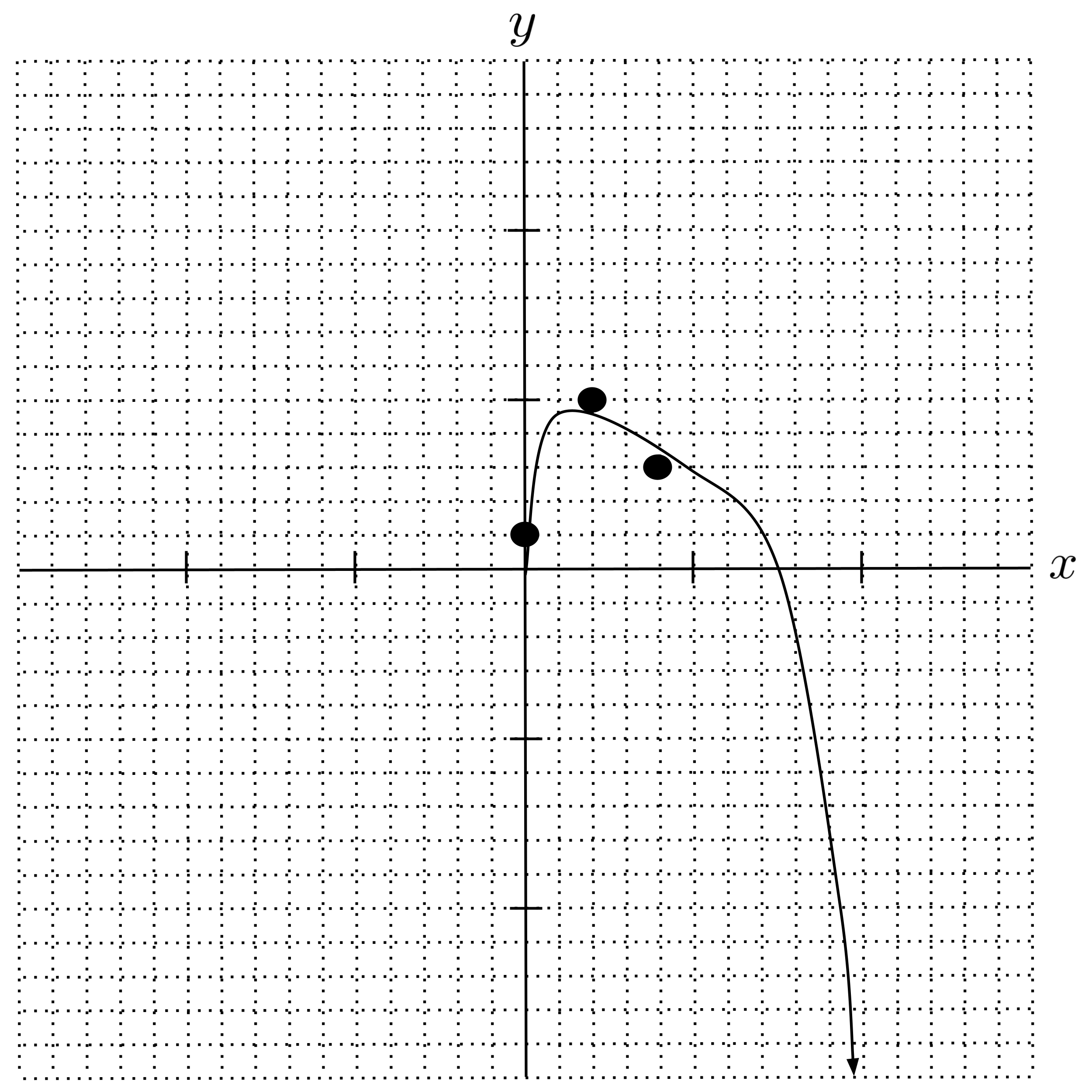
Note that $2^a$ and $\sqrt{b}$ are themselves constants, so this is in the desired general form. Let’s fit this model to the data set that we’ve been working with:

$\begin{align*} \left[ (0,1), (2,5), (4,3) \right] \end{align*}$

First, we set up our system:

$\begin{align*} (x,y) \quad &\to \quad y = \pm 2^a \cdot \dfrac{2^x}{1+x} \pm \sqrt b \cdot \dfrac{\sqrt{x}}{1 + x} \\ \\ (0,1) \quad &\to \quad 1 = \pm 2^a \cdot \dfrac{2^0}{1+0} \pm \sqrt b \cdot \dfrac{\sqrt{0}}{1 + 0} \quad \to \quad 1 = \pm 2^a \cdot 1 \pm \sqrt b \cdot 0 \\ (2,5) \quad &\to \quad 5 = \pm 2^a \cdot \dfrac{2^2}{1+2} \pm \sqrt b \cdot \dfrac{\sqrt{2}}{1 + 2} \quad \to \quad 1 = \pm 2^a \cdot \dfrac{4}{3} \pm \sqrt b \cdot \dfrac{\sqrt 2}{3} \\ (4,3) \quad &\to \quad 3 = \pm 2^a \cdot \dfrac{2^4}{1+4} \pm \sqrt b \cdot \dfrac{\sqrt{4}}{1 + 4} \quad \to \quad 1 = \pm 2^a \cdot \dfrac{16}{5} \pm \sqrt b \cdot \dfrac{2}{5} \end{align*}$

Then we convert to a matrix equation and multiply both sides by the transpose of the coefficient matrix.

$\begin{align*} \begin{bmatrix} 1 \\ 5 \\ 3 \end{bmatrix} &= \begin{bmatrix} 1 & 0 \\ 4/3 & \sqrt 2 / 3 \\ 16/5 & 2/5 \end{bmatrix} \begin{bmatrix} \pm 2^a \\ \pm \sqrt b \end{bmatrix} \\[5pt] \begin{bmatrix} 1 & 4/3 & 16/5 \\ 0 & \sqrt 2/3 & 2/5 \end{bmatrix} \begin{bmatrix} 1 \\ 5 \\ 3 \end{bmatrix} &= \begin{bmatrix} 1 & 4/3 & 16/5 \\ 0 & \sqrt 2/3 & 2/5 \end{bmatrix} \begin{bmatrix} 1 & 0 \\ 4/3 & \sqrt 2 / 3 \\ 16/5 & 2/5 \end{bmatrix} \begin{bmatrix} \pm 2^a \\ \pm \sqrt b \end{bmatrix} \end{align*}$

Finally, we evaluate the expression involving the inverse using a computer:

$\begin{align*} \begin{bmatrix} \pm 2^a \\ \pm \sqrt b \end{bmatrix} &= \left( \begin{bmatrix} 1 & 4/3 & 16/5 \\ 0 & \sqrt 2/3 & 2/5 \end{bmatrix} \begin{bmatrix} 1 & 0 \\ 4/3 & \sqrt 2 / 3 \\ 16/5 & 2/5 \end{bmatrix} \right)^{-1} \begin{bmatrix} 1 & 4/3 & 16/5 \\ 0 & \sqrt 2/3 & 2/5 \end{bmatrix} \begin{bmatrix} 1 \\ 5 \\ 3 \end{bmatrix} \\[5pt] &\approx \begin{bmatrix} -0.14 \\ 10.01 \end{bmatrix} \end{align*}$

We have the following model:

$\begin{align*} y \approx -0.14 \cdot \dfrac{2^x}{1+x} + 10.01 \cdot \dfrac{\sqrt{x}}{1 + x} \end{align*}$

Functions that Cannot be Pulled Apart

Despite the example above, not every model can be fit using the pseudoinverse method. For example, the model below cannot be fit using the pseudoinverse because there are no rules of algebra that would allow us to pull it apart:

$\begin{align*} y = \sin(ax) \cos (bx) \end{align*}$

Functions of Multiple Inputs

Finally, note that all the discussion above also generalizes to functions of multiple inputs. For example, we can apply the pseudoinverse method to fit any model of the following form:

$\begin{align*} z = a f(x,y) + b g(x,y) + c h(x,y) + \ldots \end{align*}$

To demonstrate how this works, let’s fit the model

$\begin{align*} z = ax \sin y + b y \ln (1+x) \end{align*}$

to the following data set:

$\begin{align*} \left[ (0,1,50), (2,5,30), (4,3,20), (5,1,10) \right] \end{align*}$

First, we set up our system:

$\begin{align*} (x,y,z) \quad &\to \quad z = a \cdot x \sin y + b \cdot y \ln (1+x) \\ \\ (0,1,50) \quad &\to \quad 50 = a \cdot 0 \sin 1 + b \cdot 1 \ln (1+0) \quad \to \quad 50 = a \cdot 0 + b \cdot 0 \\ (2,5,30) \quad &\to \quad 30 = a \cdot 2 \sin 5 + b \cdot 5 \ln (1+2) \quad \to \quad 30 = a \cdot 2 \sin 5 + b \cdot 5 \ln 3 \\ (4,3,20) \quad &\to \quad 20 = a \cdot 4 \sin 3 + b \cdot 3 \ln (1+4) \quad \to \quad 20 = a \cdot 4 \sin 3 + b \cdot 3 \ln 5 \\ (5,1,10) \quad &\to \quad 10 = a \cdot 5 \sin 1 + b \cdot 1 \ln (1+5) \quad \to \quad 10 = a \cdot 5 \sin 1 + b \cdot \ln 6 \end{align*}$

Then we convert to a matrix equation and multiply both sides by the transpose of the coefficient matrix.

$\begin{align*} \begin{bmatrix} 50 \\ 30 \\ 20 \\ 10 \end{bmatrix} &= \begin{bmatrix} 0 & 0 \\ 2 \sin 5 & 5 \ln 3 \\ 4 \sin 3 & 3 \ln 5 \\ 5 \sin 1 & \ln 6 \end{bmatrix} \begin{bmatrix} a \\ b \end{bmatrix} \\[5pt] \begin{bmatrix} 0 & 2 \sin 5 & 4 \sin 3 & 5 \sin 1 \\ 0 & 5 \ln 3 & 3 \ln 5 & \ln 6 \end{bmatrix} \begin{bmatrix} 50 \\ 30 \\ 20 \\ 10 \end{bmatrix} &= \begin{bmatrix} 0 & 2 \sin 5 & 4 \sin 3 & 5 \sin 1 \\ 0 & 5 \ln 3 & 3 \ln 5 & \ln 6 \end{bmatrix} \begin{bmatrix} 0 & 0 \\ 2 \sin 5 & 5 \ln 3 \\ 4 \sin 3 & 3 \ln 5 \\ 5 \sin 1 & \ln 6 \end{bmatrix} \begin{bmatrix} a \\ b \end{bmatrix} \end{align*}$

Finally, we evaluate the expression involving the inverse using a computer:

$\begin{align*} \begin{bmatrix} a \\ b \end{bmatrix} &= \left( \begin{bmatrix} 0 & 2 \sin 5 & 4 \sin 3 & 5 \sin 1 \\ 0 & 5 \ln 3 & 3 \ln 5 & \ln 6 \end{bmatrix} \begin{bmatrix} 0 & 0 \\ 2 \sin 5 & 5 \ln 3 \\ 4 \sin 3 & 3 \ln 5 \\ 5 \sin 1 & \ln 6 \end{bmatrix} \right)^{-1} \begin{bmatrix} 0 & 2 \sin 5 & 4 \sin 3 & 5 \sin 1 \\ 0 & 5 \ln 3 & 3 \ln 5 & \ln 6 \end{bmatrix} \begin{bmatrix} 50 \\ 30 \\ 20 \\ 10 \end{bmatrix} \\[5pt] &\approx \begin{bmatrix} -0.13 \\ 4.93 \end{bmatrix} \end{align*}$

We have the following model:

$\begin{align*} z \approx -0.13 \, x \sin y + 4.93 \, y \ln (1+x) \end{align*}$

Exercises

Use the pseudoinverse method to fit each model to the given data set. Check your answer each time by sketching the resulting model on a graph containing the data points and verifying that it visually appears to capture the trend of the data.

Fit $y = a \ln (1 + x) + \dfrac{b}{x}$ to $[(1,0), (3,-1), (4,5)].$
Fit $y = \dfrac{ax + b}{2^x}$ to $[(1,0), (3,-1), (4,5)].$
Fit $y = \pm 3^{a + x} \pm \sqrt[3]{bx}$ to $[(1,0), (3,-1), (4,5)].$
Fit $z = a xy^2 + b \cdot 2^{x + y}$ to $[(-2,3,-3), (1,0,-4), (3,-1,2), (4,5,3)].$