Regression via Gradient Descent

by Justin Skycak on January 05, 2022

Gradient descent can help us avoid pitfalls that occur when fitting nonlinear models using the pseudoinverse.

This post is a chapter in the book Introduction to Algorithms and Machine Learning: from Sorting to Strategic Agents. Suggested citation: Skycak, J. (2022). Regression via Gradient Descent. Introduction to Algorithms and Machine Learning: from Sorting to Strategic Agents. https://justinmath.com/regression-via-gradient-descent/

Gradient descent can be applied to fit regression models. In particular, it can help us avoid the pitfalls that we’ve experienced when we attempt to fit nonlinear models using the pseudoinverse.

Previously, we fit a power regression $y = ax^b$ to the following data set and got a result that was quite obviously not the most accurate fit.

$\begin{align*} \left[ (0.001, 0.01), (2,4), (3,9) \right] \end{align*}$

This time, we will use gradient descent to fit the power regression and observe that our resulting model fits the data much better.

Model-Fitting as a Minimization Problem

To fit a model using gradient descent, we just have to construct an expression that represents the error between the model and the data that it’s supposed to fit. Then, we can use gradient descent to minimize that expression.

To represent the error between the model and the data that it’s supposed to fit, we can use the residual sum of squares (RSS). To compute the RSS, we just add up the squares of the differences between the model’s predictions and the actual data.

$\begin{align*} \textrm{data point} \quad &\to \quad \textrm{predicted } y\textrm{-value} &\textrm{vs} \quad &\textrm{data } y\textrm{-value} \\ (x,y) \quad &\to \quad ax^b &\textrm{vs} \quad & y \\ \\ (0.001, 0.01) \quad &\to \quad a \cdot (0.001)^b &\textrm{vs} \quad & 0.01 \\ (2, 4) \quad &\to \quad a \cdot 2^b &\textrm{vs} \quad & 4 \\ (3, 9) \quad &\to \quad a \cdot 3^b &\textrm{vs} \quad & 9 \end{align*}$

Summing up the squared differences between the predicted $y$-values and the $y$-values in the data, we get the following expression for the RSS:

$\begin{align*} \textrm{RSS} = \left( a \cdot (0.001)^b - 0.01 \right)^2 + \left( a \cdot 2^b - 4 \right)^2 + \left( a \cdot 3^b - 9 \right)^2 \end{align*}$

Now, this is a normal gradient descent problem. We choose an initial guess for $a$ and $b$ and then use the partial derivatives $\frac{\partial \textrm{RSS}}{\partial a}$ and $\frac{\partial \textrm{RSS}}{\partial b}$ to repeatedly update our guess so that it results in a lower RSS.

Computing partial derivatives, we have the following:

$\begin{align*} \dfrac{\partial \textrm{RSS}}{\partial a} &= 2\left( a \cdot (0.001)^b - 0.01 \right) (0.001)^b \\ &\phantom{=}+ 2\left( a \cdot 2^b - 4 \right) \cdot 2^b \\ &\phantom{=}+ 2\left( a \cdot 3^b - 9 \right) \cdot 3^b \\[5pt] \dfrac{\partial \textrm{RSS}}{\partial b} &= 2\left( a \cdot (0.001)^b - 0.01 \right) \cdot a \cdot (0.001)^b \ln (0.001) \\ &\phantom{=}+ 2\left( a \cdot 2^b - 4 \right) \cdot a \cdot 2^b \ln 2 \\ &\phantom{=}+ 2\left( a \cdot 3^b - 9 \right) \cdot a \cdot 3^b \ln 3 \end{align*}$

Worked Example

Let’s start with the initial guess $\left< a_0, b_0 \right> = \left< 1, 1 \right>,$ which corresponds to the straight line $y = 1x^1.$ Our gradient is

$\begin{align*} \nabla \textrm{RSS}(a_0, b_0) &= \left. \left< \dfrac{\partial \textrm{RSS}}{\partial a}, \dfrac{\partial \textrm{RSS}}{\partial b} \right> \right|_{(a_0, b_0)} \\[5pt] &= \left< -44.000018, -45.095095 \right>, \end{align*}$

and using learning rate $\alpha = 0.001$ our updated guess is

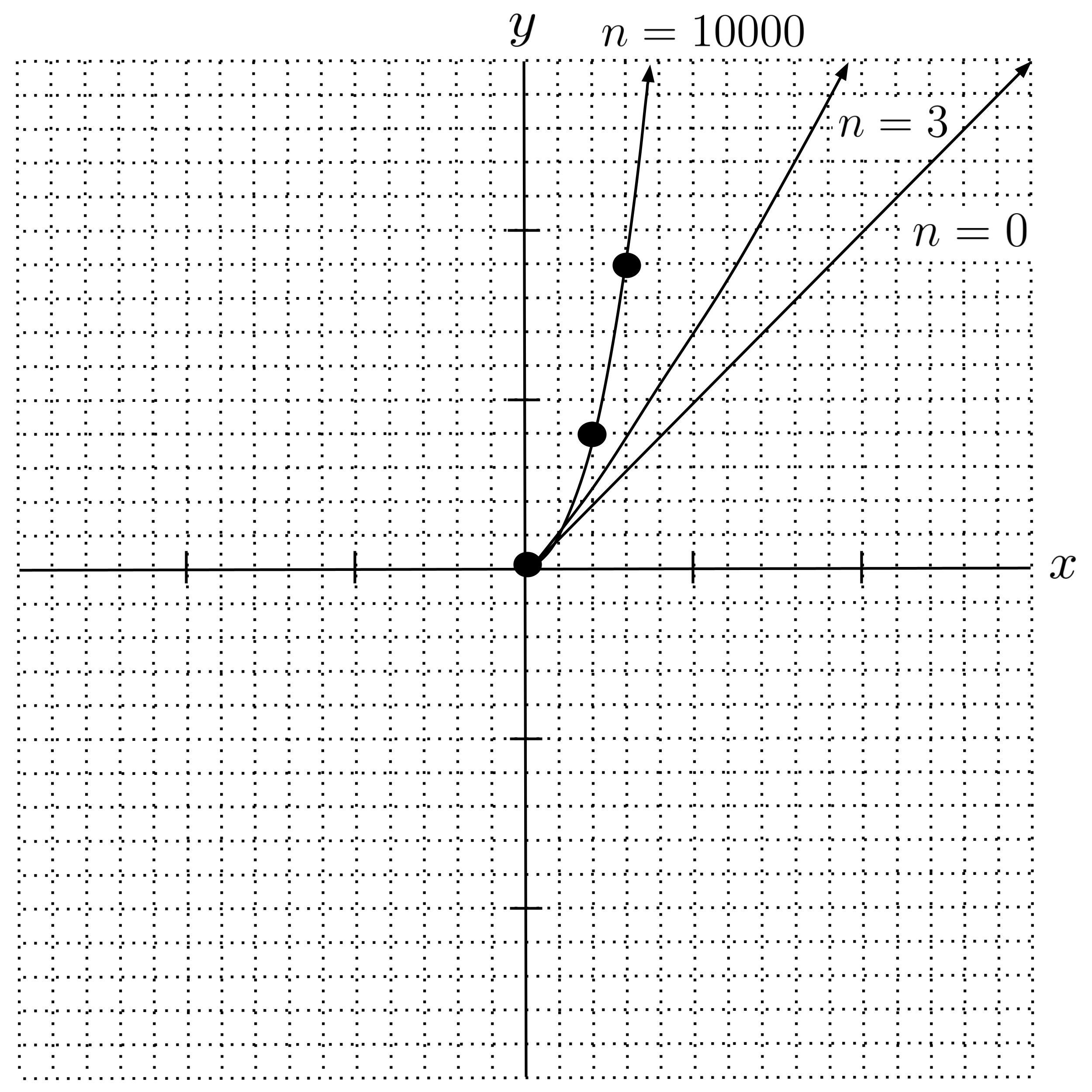
$\begin{align*} \left< a_1, b_1 \right> &= \left< a_0, b_0 \right> - \alpha \nabla \textrm{RSS}(a_0, b_0) \\[5pt] &= \left< 1,1 \right> - (0.001) \left< -44.000018, -45.095095 \right> \\[5pt] &= \left< 1.044000, 1.045095 \right>. \end{align*}$

If we continue the process, we get the results shown in the table below.

$\begin{align*} \begin{matrix} n & \left< a_n, b_n \right> & \nabla \textrm{RSS}(a_n,b_n) & \big\vert & \textrm{RSS}(a_n, b_n) \\ \hline 0 & \left< 1, 1 \right> & \left< -44.000018, -45.095095 \right> & \big\vert & 40.000081 \\ 1 & \left< 1.044000, 1.045095 \right> & \left< -43.610529, -46.794623 \right> & \big\vert & 35.998548 \\ 2 & \left< 1.087611, 1.091890 \right> & \left< -42.948407, -48.155772 \right> & \big\vert & 31.88666 \\ 3 & \left< 1.130559, 1.140045 \right> & \left< -41.947662, -49.053128 \right> & \big\vert & 27.719376 \\ 50 & \left< 1.450958, 1.640770 \right> & \left< 0.849948, -0.569792 \right> & \big\vert & 0.315108 \\ 100 & \left< 1.410093, 1.668529 \right> & \left< 0.783786, -0.539881 \right> & \big\vert & 0.266312 \\ 500 & \left< 1.185035, 1.836774 \right> & \left< 0.378140, -0.307757 \right> & \big\vert & 0.061737 \\ 1000 & \left< 1.065472, 1.939139 \right> & \left< 0.137242, -0.123755 \right> & \big\vert & 0.008426 \\ 5000 & \left< 1.000014, 1.999987 \right> & \left< -0.000029, -0.000028 \right> & \big\vert & 0.000100 \\ 10000 & \left< 1.000000, 2.000000 \right> & \left< 0.000000, 0.000000 \right> & \big\vert & 0.000100 \\ \end{matrix} \end{align*}$

Our gradient descent converged to $a=1$ and $b=2,$ which corresponds to the function $y = 1x^2.$ As we can see from the graph below, this is a very good fit.

Sigma Notation and Implementation

Note that when implementing gradient descent on a data set consisting of more than a few points, it becomes infeasible to hard-code the entire expression for the RSS gradient. Instead, it becomes necessary to write a function that loops through the points in the data set and incrementally adds up each point’s individual contribution to the total RSS gradient. It also becomes convenient to re-use intermediate values when possible.

To think through this, it’s helpful to express the RSS and its gradient using sigma notation. In the example above, the RSS is given by

$\begin{align*} \textrm{RSS} = \sum\limits_{(x,y) \, \in \, \textrm{data}} \left( a x^b - y \right)^2, \end{align*}$

and its gradient is computed as

$\begin{align*} \nabla \textrm{RSS} &= \sum\limits_{(x,y) \, \in \, \textrm{data}} \nabla \left( a x^b - y \right)^2 \\[5pt] &= \sum\limits_{(x,y) \, \in \, \textrm{data}} 2\left( a x^b - y \right) \nabla \left( a x^b - y \right) \\[5pt] &= \sum\limits_{(x,y) \, \in \, \textrm{data}} 2\left( a x^b - y \right) \left< \dfrac{\partial}{\partial a} \left( a x^b - y \right), \dfrac{\partial}{\partial b} \left( a x^b - y \right) \right> \\[5pt] &= \sum\limits_{(x,y) \, \in \, \textrm{data}} 2\left( a x^b - y \right) \left< x^b, abx^{b-1} \right> \\[5pt] &= \sum\limits_{(x,y) \, \in \, \textrm{data}} 2\left( a x^b - y \right) x^b \left< 1, abx^{-1} \right>. \end{align*}$

Now that we’ve worked out the sigma notation, we can write a function that mirrors it:


gradRSS(a, b, data):
    da = 0
    db = 0
    for (x,y) in data:
        common = 2 * (ax^b - y) * x^b
        da += common
        db += common * a * b * x^-1
    return da, db

Debugging with Central Difference Quotients

Lastly, note that when debugging broken gradient descent code, it can be helpful to check your partial derivatives against difference quotient approximations to ensure that you’re computing the partial derivatives correctly:

$\begin{align*} \dfrac{\partial \textrm{RSS}}{\partial a} &\approx \dfrac{\textrm{RSS}(a + h, b) - \textrm{RSS}(a - h, b)}{2h} \\[5pt] \dfrac{\partial \textrm{RSS}}{\partial b} &\approx \dfrac{\textrm{RSS}(a, b+h) - \textrm{RSS}(a, b-h)}{2h} \end{align*}$

where $0 < h \ll 1$ is a small positive number.

Do not abuse difference quotients and attempt to use them to fully bypass gradient computations. Use difference quotients only for debugging. Difference quotients will be too slow to effectively train more advanced models (such as neural networks), and it’s useful to practice gradient computations on simpler models before moving on to more advanced models.

Exercises

Use gradient descent to fit the following models. Be sure to plot your model on the same graph as the data to ensure that the fit is looks reasonable.

Implement the example that was worked out above.
Fit $y = ax^2 + bx + c$ to $\left[ (0.001, 0.01), (2,4), (3,9) \right].$ Verify that gradient descent gives the same fit as compared to using the pseudoinverse.
Fit $y = \dfrac{5}{1+e^{-(ax+b)}} + 0.5$ to $[(1,1), (2,1), (3,2)].$ Verify that gradient descent gives a better fit as compared to using the pseudoinverse.
Fit $y = a \sin bx + c \sin dx$ to
$\begin{align*} \begin{bmatrix} \left(0,0\right), & \left(1,-1\right), &\left(2,2\right), &\left(3,0\right), &\left(4,0\right) \\ \left(5,2\right), &\left(6,-4\right), &\left(7,4\right), &\left(8,1\right), &\left(9,-3\right) \end{bmatrix}. \end{align*}$