Reimplementing Fogel’s Tic-Tac-Toe Paper

by Justin Skycak on March 05, 2022

Reimplementing the paper that laid the groundwork for Blondie24.

This post is a chapter in the book Introduction to Algorithms and Machine Learning: from Sorting to Strategic Agents. Suggested citation: Skycak, J. (2022). Reimplementing Fogel's Tic-Tac-Toe Paper. Introduction to Algorithms and Machine Learning: from Sorting to Strategic Agents. https://justinmath.com/reimplementing-fogels-tic-tac-toe-paper/

The goal of this chapter is to reimplement the paper Using Evolutionary Programming to Create Neural Networks that are Capable of Playing Tic-Tac-Toe by David Fogel in 1993. This paper preceded Blondie24, and many of the principles introduced in this paper were extended in Blondie24. As such, reimplementing the paper provides good scaffolding as we work our way up to reimplement Blondie24.

The information needed to reimplement this paper is outlined below.

Neural Network Architecture

The neural net consists of the following layers:

Input Layer: $9$ linearly-activated nodes and $1$ bias node
Hidden Layer: $H$ sigmoidally-activated nodes and $1$ bias node ($H$ is variable, as will be described later)
Output Layer: $9$ sigmoidally-activated nodes

Converting Board to Input

A tic-tac-toe board is converted to input by flattening it into a vector and replacing $\textrm X$ with $1,$ empty squares with $0,$ and $\textrm O$ with $-1.$

For example, given a board

$\begin{align*} \begin{bmatrix} \textrm{X} & \textrm{O} & \square \\ \square & \textrm{X} & \textrm{O} \\ \square & \square & \square \end{bmatrix}, \end{align*}$

we first concatenate consecutive rows to flatten the board into the following $9$-element vector:

$\begin{align*} \left< \textrm{X}, \textrm{O}, \square, \square, \textrm{X}, \textrm{O}, \square, \square, \square \right>, \end{align*}$

Then, we replace $\textrm X$ with $1,$ empty squares with $0,$ and $\textrm O$ with $-1$ to get the final input vector:

$\begin{align*} \left< 1, -1, 0, 0, 1, -1, 0, 0, 0 \right> \end{align*}$

Converting Output to Action

The output layer consists of $9$ nodes, one for each board square. To convert the output values into an action, we do the following:

Discard any values that correspond to a board square that has already been filled. (This will prevent illegal moves.)
Identify the empty board square with the maximum value. We move into this square.

Evolution Procedure

The initial population consists of $50$ networks. In each network, the number of hidden nodes $H$ is randomly chosen from the range ${ 1, 2, \ldots, 10 }$ and the initial weights are randomly chosen from the range $[-0.5, 0.5].$

Replication

A network replicates by making a copy of itself and then modifying the copy as follows:

Each weight is incremented by $N(0,0.05^2),$ a value drawn from the normal distribution with mean $0$ and standard deviation $0.05.$
With $0.5$ probability, we modify the network architecture. If we modify the architecture, then we do so by randomly choosing between adding or deleting a hidden node. If we add a node, then we initialize its associated weights with values of $0.$

Note that when modifying the architecture, we abort any decision that would lead the number of hidden nodes to exit the range ${ 1, 2, \ldots, 10 }.$ More specifically:

We abort the decision to delete a hidden node if the number of hidden nodes is $H=1.$
We abort the decision to add a hidden node if the number of hidden nodes is $H=10.$

Evaluation

In each generation, each network plays $32$ games against a near-perfect but beatable opponent. The evolving network is always allowed to move first, and receives a payoff of $1$ for a win, $0$ for a tie, and $-10$ for a loss.

The near-perfect opponent follows the strategy below:


With 10% chance:
 - Randomly choose an open square to move into.

Otherwise:
 - If the next move can be chosen to win the game, do so.

 - Otherwise, if the next move can be chosen to block
   the opponent's win, do so.

 - Otherwise, if there are 2 open squares in a line with
   the opponent's marker, randomly move into one of those
   squares.

 - Otherwise, randomly choose an open square to move into.

Once the total payoff (over $32$ games against the near-perfect opponent) has been computed for each of the $100$ networks (the $50$ parents and their $50$ children), a second round of evaluation occurs to select the networks that will proceed to the next generation and replicate.

In the second round of evaluation, each network is given a score that represents how its total payoff (from matchups with the near-perfect opponent) compares to the total payoffs of some other networks in the same generation. Specifically, each network is compared to $10$ other networks randomly chosen from the generation, and its score is incremented for each other network that has a lower total payoff.

The top $50$ networks from the second round of evaluation are selected to proceed to the next generation and replicate.

Note: The actual paper states that the networks with the highest performance from the second round of evaluation are selected. Interpreted formally, it would suggest to only select those network(s) that had the absolute maximum performance. But this would lead the generations to rapidly shrink in size, resulting in premature convergence. The informal interpretation (top $50$ networks) leads the generation sizes to stay the same, which avoids the issue.

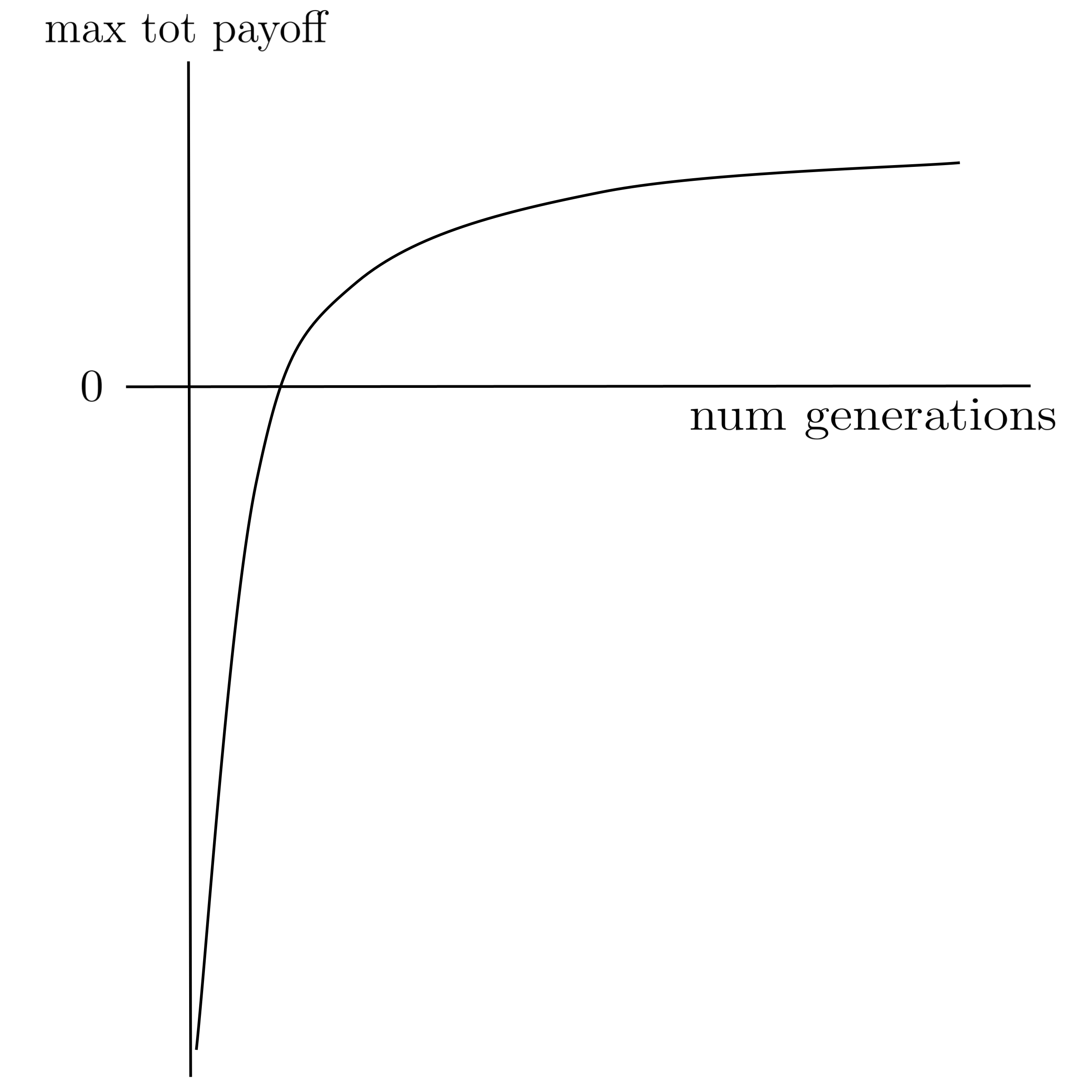
Performance Curve

Generate a performance curve as follows:

Run the above procedure for $800$ generations, keeping track of the maximum total payoff (i.e. the best player's total payoff) at each generation.
Then repeat $19$ more times, for a total of $20$ trials of $800$ generations each.
Finally, plot the mean maximum total payoff (averaged over the $20$ trials) as a function of the number of generations.

The resulting curve should resemble the following shape:

Once you’re able to generate a good performance curve, store the neural network parameters for the best player from the last generation so that you can play it against a random player and verify its intelligence. (It should beat the random player the vast majority of the time.)

Debugging

Before you attempt to run the full $20$ trials of $800$ generations with $50$ parent networks in each generation, run a quicker sanity check (say, $5$ trials of $50$ generations with $10$ parent networks in each generation) to make sure that the curve looks like it’s moving in the correct direction (upward).

Given the complexity of this project, your plot will likely not come out correct the first time you try to run it, even if you feel certain that you have correctly implemented the specifications of the paper.

If and when this happens, you will need to add plenty of validation to your implementation. A non-exhaustive list of validation checks and unit tests are provided below for the first half of the paper specifications. You will need to come up validation checks for the second half on your own.

Each generation, check that each individual neural network has a valid number of nodes in each layer.
Whenever you convert a board to input for a neural network, check that the resulting entries are all in the set $\{ -1, 0, 1 \}$ add up to $0$ before the neural network player makes its next move.
Create a unit test takes a variety of possible board states and output vectors from the neural network and then verifies that the player makes the appropriate move.
Check that the initial weights are between $-0.5$ and $0.5,$ no weight stays the same after replication, some weights increase and some weights decrease after replication (i.e. they don't all move in the same direction), and no weight changes by more than $0.3$ (which is $6$ standard deviations).
Check that after replication, some networks have an additional hidden layer node, other networks have one less hidden layer node, and other networks have an unchanged number of hidden layer nodes.
...

If the plot still doesn’t look right even after your sanity checks are implemented and passing, then create a log of the results using the template shown below.

(Sometimes there can be issues that you don’t anticipate in your sanity checks, that become apparent when you take a birds-eye view and manually look at concrete numbers.)


HYPERPARAMETERS
   Networks per generation: 20
   Selection percentage: 0.5

ABBREVIATIONS
   star (*) if selected
   H = number of non-bias neurons in hidden layer
   [min weight, mean weight, max weight]
   (wins : losses : ties)
   (IDs won against | IDs lost against | IDs tied against)

GENERATION 1

  NN 1 (parent, H=7, [-0.42, 0.02, 0.37])
    payoff -300  (0:30:2)
    score 2  (7,17|2,7,16,12,13|8,11,19)
  
* NN 2 (parent, H=3, [-0.49, -0.05, 0.45])
    payoff -190  (10:20:2)
    score=7  (3,8,9,11,12,14,19|15|4,10)
    
  ...
  
* NN 20 (child of 10, H=5, [-0.45, 0.03, 0.48])
    payoff -200  (10:21:1)
    score 8  (7,17|2,7,16,12,13|8,11,19)]

GENERATION 2

  NN 2 (parent, ...)
    payoff ...
    score ...
    
* NN 4 (parent, ...)
    payoff ...
    score ...

  ...

  NN 20 (parent, ...)
    payoff ...
    score ...

* NN 21 (child of 2, ...)
    payoff ...
    score ...
  
  NN 40 (child of 20, ...)
    payoff ...
    score ...
    
  ...