Introduction to Blondie24 and Neuroevolution

by Justin Skycak on March 04, 2022

A method for training neural networks that works even when training feedback is sparse.

This post is a chapter in the book Introduction to Algorithms and Machine Learning: from Sorting to Strategic Agents. Suggested citation: Skycak, J. (2022). Introduction to Blondie24 and Neuroevolution. Introduction to Algorithms and Machine Learning: from Sorting to Strategic Agents. https://justinmath.com/introduction-to-blondie24-and-neuroevolution/

Previously, we built strategic connect four players by constructing a pruned game tree, using heuristics to rate terminal states, and then applying the minimax algorithm. This was a combination of game-specific human intelligence (heuristics) and generalizable artificial intelligence (minimax on a game tree).

Blondie24

In the 1990s, a researcher named David Fogel managed to automate the process of rating states in pruned game trees without relying on heuristics or any other human input. In particular, he and his colleague Kumar Chellapilla created a computer program that achieved expert level checkers-playing ability by learning from scratch. They played it against other humans online under the username Blondie24, pretending to be a 24-year old blonde female college student.

Blondie24 was particularly noteworthy because other successful game-playing agents had been hand-tuned and/or trained on human-expert strategies. Unlike these agents, Blondie24 learned without having any access to information on human-expert strategies.

To automate the process of rating states in pruned game trees, Fogel turned it into a regression problem: given a game state, predict its value. Of course, the regression function is pretty complicated (e.g. changing one piece on a chess board can totally change the outcome of the game), so the natural choice was to use a neural network.

However, the usual method of training a neural network, backpropagation, does not work in this setting. Backpropagation relies on a dataset of pairs of inputs and outputs – which means that the model would need a data set of game states along with their correct rating, totally defeating the purpose of getting the model to learn this information from scratch. In this setting, the only feedback the computer gets is at the very end of the game, whether it won or lost (or tied).

Neuroevolution

To get around this issue, Fogel trained neural networks via evolution, which is often referred to as neuroevolution in the context of neural networks. Starting with a population of many neural networks with random weights, he repeatedly

played the networks against each other,
discarded the networks that performed worse than average,
duplicated the remaining networks, and then
randomly perturbed the weights of the duplicate networks.

This is analogous to the concept of evolution in biology in which weak organisms die and fit organisms survive to produce similar but slightly mutated offspring. By repeatedly running the evolutionary procedure, Fogel was able to evolve a neural network whose internal mapping from input state to output rating caused it to play the game of checkers in an intelligent way, without any sort of human input.

Exercise: Evolving a Neural Network Regressor

Before we reimplement Fogel’s papers leading up to Blondie24, let’s first gain some experience with neuroevolution in a simpler case. As a toy problem, consider the following data set:


[
  (0.0, 1.0), (0.04, 0.81), (0.08, 0.52), (0.12, 0.2), (0.17, -0.12),
  (0.21, -0.38), (0.25, -0.54), (0.29, -0.58), (0.33, -0.51), (0.38, -0.34),
  (0.42, -0.1), (0.46, 0.16), (0.5, 0.39), (0.54, 0.55), (0.58, 0.61),
  (0.62, 0.55), (0.67, 0.38), (0.71, 0.12), (0.75, -0.19), (0.79, -0.51),
  (0.83, -0.77), (0.88, -0.95), (0.92, -1.0), (0.96, -0.91), (1.0, -0.7)
]

We will fit the above data using a neural network regressor with the following architecture:

Input Layer: $1$ linearly-activated node and $1$ bias node
First Hidden Layer: $10$ tanh-activated nodes and $1$ bias node
Second Hidden Layer: $6$ tanh-activated nodes and $1$ bias node
Third Hidden Layer: $3$ tanh-activated nodes and $1$ bias node
Output Layer: $1$ tanh-activated node

Remember that hyperbolic tangent function is defined as

$\begin{align*} \tanh x = \dfrac{e^x - e^{-x}}{e^x + e^{-x}}. \end{align*}$

To train the neural network, use the following evolutionary algorithm (which is based on the Blondie24 approach):

Create a population of $15$ neural networks with weights randomly drawn from $[-0.2, 0.2].$ Additionally, assign a mutation rate to each net, initially equal to $\alpha = 0.05.$
Each of the $15$ parents replicates to produce a single child. The child is given mutation rate $\begin{align*} \alpha^\text{child} = \alpha^\text{parent} e^{ N(0,1) / \sqrt{ 2 \sqrt{|W|}} } \end{align*}$
and weights

$\begin{align*} w_{ij}^\text{child} = w_{ij}^\text{parent} + \alpha^\text{child} N(0,1), \end{align*}$
where $N(0,1)$ is a random number drawn from the standard normal distribution and $|W|$ is the number of weights in the network. Be sure to draw a different random number for each instance of $N(0,1).$
Compute the RSS for each net and select the $15$ nets with the lowest RSS. These will be the parents in the next generation.
Go back to step 2.

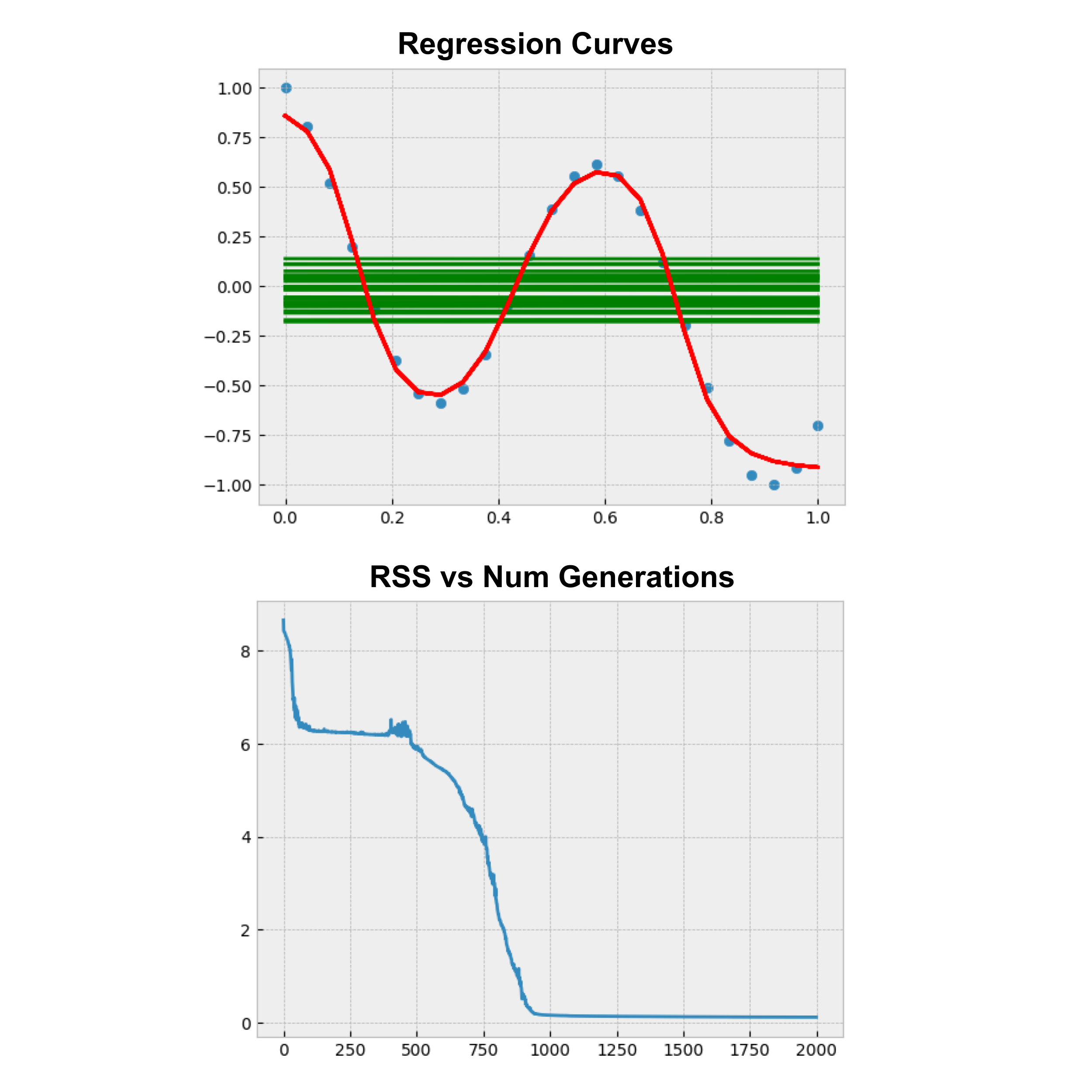
Make a plot of the average RSS at each generation, run the algorithm until the graph levels off to nearly $0,$ and then plot the regression curves corresponding to the first and last generations of neural networks on a graph along with the data.

(The regression curve plot will contain $60$ different curves drawn on the same plot: one curve from each of the $30$ nets in the first generation, and one curve from each of the $30$ nets in the last generation.)

The first generation curves will not fit the data at all (they will appear flat), but the final generation of regression curves should fit the data remarkably well. Note that the training process may require on the order of a thousand generations.

Exercise: Hyperparameter Tuning

Once you’ve got this working, try tuning hyperparameters to get the RSS to converge to nearly $0$ as quickly as possible. You can tweak the mutation rate, initial weight distribution, number of neural networks, and neural network architecture (i.e. number of hidden layers and their sizes).

Visualizations

Courtesy of Maia Dimas, below is an illustration of the first and last generations of neural nets, along with a graph of RSS versus the number of generations.

Courtesy of Elias Gee, below is an animation of a small population ($10$ nets) as they learn to fit the curve over many generations.