Linear, Polynomial, and Multiple Linear Regression via Pseudoinverse
Using matrix algebra to fit simple functions to data sets.
This post is part of the book Introduction to Algorithms and Machine Learning: from Sorting to Strategic Agents. Suggested citation: Skycak, J. (2022). Linear, Polynomial, and Multiple Linear Regression via Pseudoinverse. In Introduction to Algorithms and Machine Learning: from Sorting to Strategic Agents. https://justinmath.com/linear-polynomial-and-multiple-linear-regression-via-pseudoinverse/
Want to get notified about new posts? Join the mailing list and follow on X/Twitter.
Supervised learning consists of fitting functions to data sets. The idea is that we have a sample of inputs and outputs from some process, and we want to come up with a mathematical model that predicts what the outputs would be for other inputs. Supervised machine learning involves programming computers to compute such models.
Linear Regression and the Pseudoinverse
One of the simplest ways to construct a predictive algorithm is to assume a linear relationship between the input and output. Even if this assumption isn’t correct, it’s always useful to start with a linear model because it provides a baseline against which we can compare the accuracy of more complicated models. (We can only justify using a complicated model if it is significantly more accurate than a linear model.)
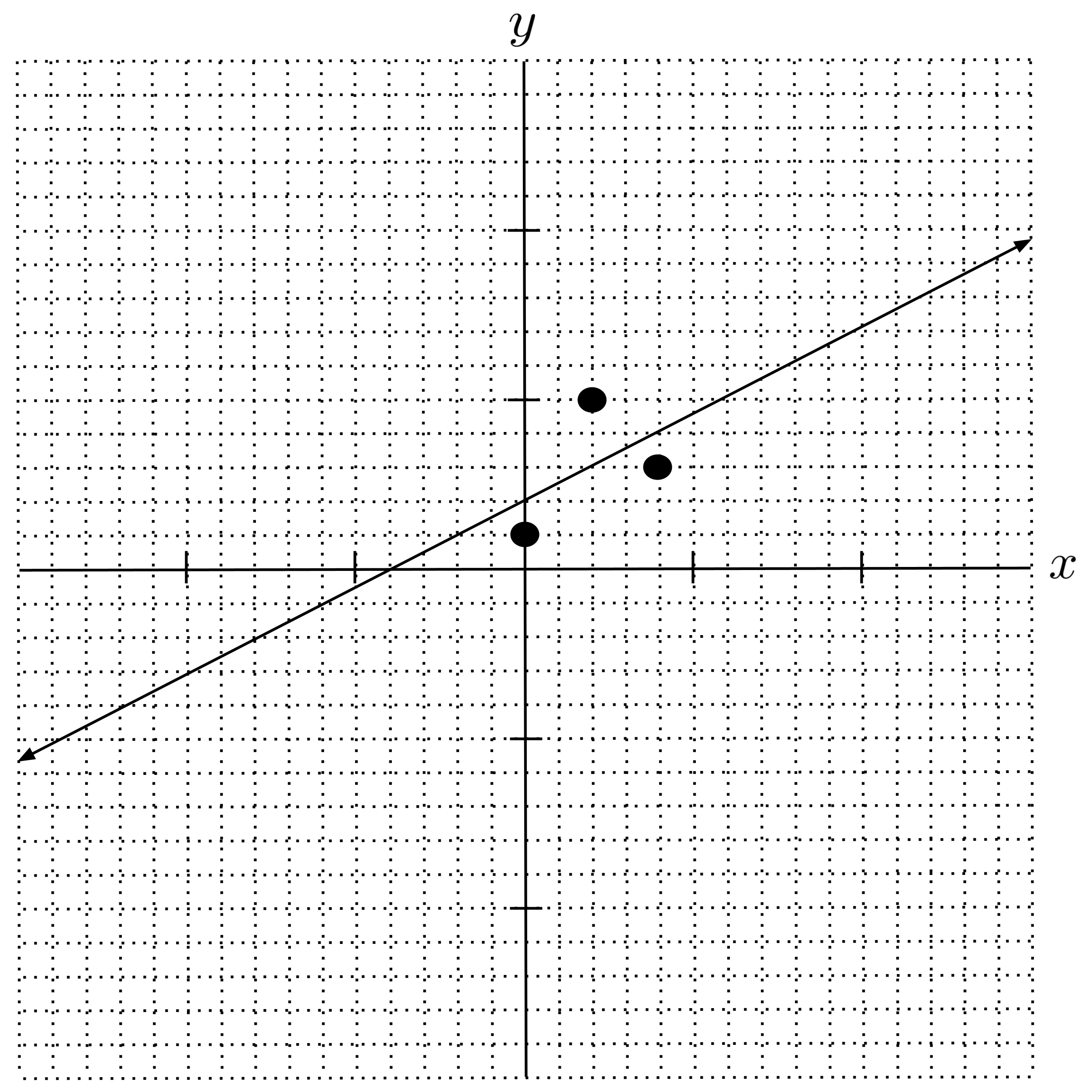
For example, let’s fit a linear model $y=mx + b$ to the following data set. That is, we want to find the values of $m$ and $b$ so that the line $y=mx+b$ most accurately represents the following data set.
While there is no single line that goes through all three points in the data set, we can choose the slope $m$ and intercept $b$ so that the line represents the data as accurately as possible. There are a handful of ways to accomplish this, the simplest of which involves leveraging the pseudoinverse from linear algebra.
To start, let’s set up the system of equations that would need to be satisfied in order for our model to have perfect accuracy on the data set. We do this by simply taking each point $(x,y)$ in our data set and plugging it into the model $y=mx+b.$
Now, we rewrite the above system using matrix notation:
You may be tempted to solve the matrix equation by inverting the coefficient matrix that’s multiplying the unknown:
Then you might remember that the inverse of a non-square matrix does not exist, and think that this was all fruitless.
But really, this is the main idea of the pseudoinverse method. The only difference is that before inverting the coefficient matrix, we multiply both sides of the equation by the transpose of the coefficient matrix so that it becomes square.
Geometrically, multiplying by the transpose takes the matrices involved in the equation and projects them onto the nearest subspace where a solution exists. This means we can now take the inverse:
Reading off the parameters $m = \dfrac{1}{2}$ and $b=2,$ we have the following linear model:
Polynomial Regression
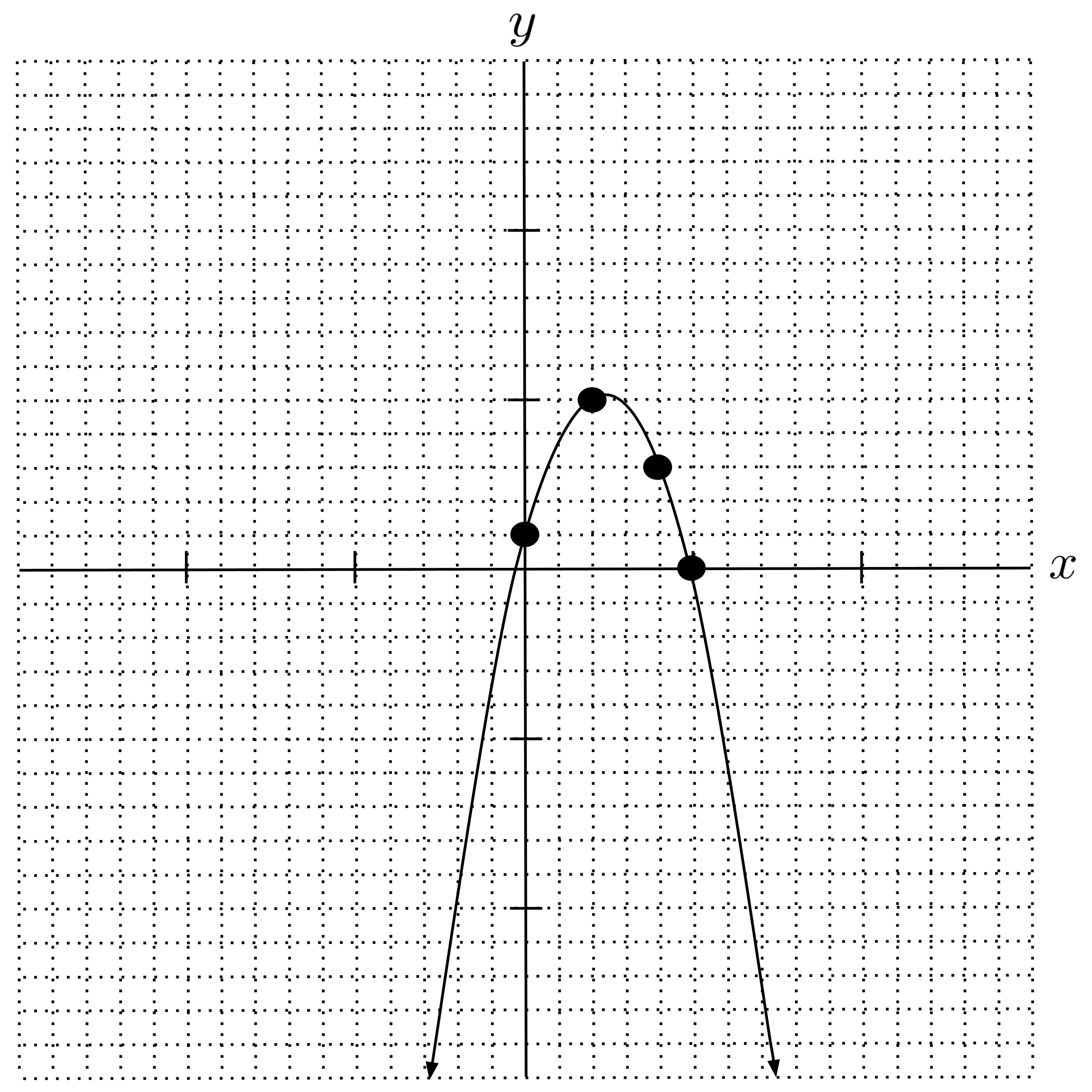
We can use the pseudoinverse method to fit polynomial models as well. To illustrate, let’s fit a quadratic model $y = ax^2 + bx + c$ to the following data set:
First, we set up our system of equations:
Then we convert to a matrix equation, multiply both sides by the transpose of the coefficient matrix, and invert the resulting square matrix.
Note that we used a computer to simplify the final step. You can start to see why computers are essential in machine learning (and this is just the tip of the iceberg).
We have the following quadratic model:
Multiple Linear Regression
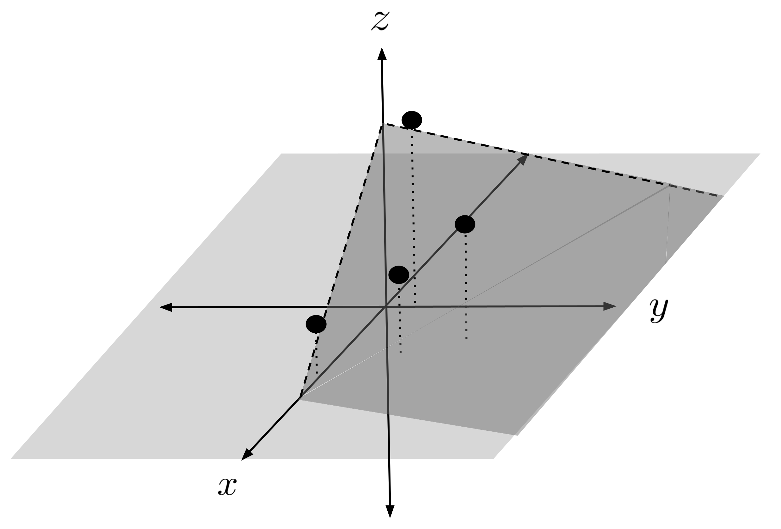
Lastly, the pseudoinverse method can also be used to fit models consisting of multiple input variables. For example, let’s fit a linear model $z = ax + by + c$ to the following data set:
Here, we have two input variables, $x$ and $y.$ Our output variable is $z.$
As usual, we begin by setting up our system of equations:
Then we convert to a matrix equation, multiply both sides by the transpose of the coefficient matrix, and invert the square matrix that results.
So, we have the following model which represents a plane in $3$-dimensional space:
When the Pseudoinverse Fails
Note that the pseudoinverse method requires that the columns of the coefficient matrix be independent. Otherwise, when we multiply by the transpose, the result is not guaranteed to be invertible. In particular, this means that the number of parameters of the model that we want to fit (i.e. the width of the coefficient matrix) should not exceed the number of distinct data points in our data set (i.e. the height of the coefficent matrix).
To illustrate what happens when the number of parameters of the model exceeds the number of distinct data points, let’s trying to fit a line $y=mx+b$ to a data set $[(2,3)]$ consisting of only a single point. (The line has $2$ parameters, $m$ and $b.$)
Although multiplying by the transpose gives us a square matrix, the square matrix is not invertible. This happens because there are infinitely many lines that have pass through the point $(2,3)$ and therefore have perfect accuracy on the data set.
General Formula
Looking back at our work, we can write down the general procedure as follows, where $y$ is the vector of outputs, $X$ is the coefficients matrix of our system of equations, and $p$ is the vector of model parameters.
The pseudoinverse of the matrix $X$ is defined by $(X^T X)^{-1} X^T,$ as shown in the last row of the general equation. To understand why this quantity is called the pseudoinverse, first recall that if we attempt to solve the equation $y = Xp$ using the regular matrix, then we get a solution of the form
The issue that we run into is that the regular inverse $X^{-1}$ usually does not exist (because $X$ is usually a tall rectangular matrix, not a square matrix). The best approximation of the solution is
which takes a similar form to the previous equation, except that the inverse $X^{-1}$ is replaced by the pseudoinverse $(X^T X)^{-1} X^T.$
Final Remarks
Finally, note that quantitative models are usually referred to as regression models when the goal is to predict some numeric value. This is contrasted with classification models, where the goal is to predict the category or class that best represents an input. So far, we have only encountered regression models, but we will learn about classification models soon.
Exercises
Use the pseudoinverse method to fit the given model to the given data set. Check your answer by sketching the resulting model on a graph containing the data points and verifying that it visually appears to capture the trend of the data. Remember that the model does not need to actually pass through all the data points (this is usually impossible).
- Fit $y = mx + b$ to $[(1,0), (3,-1), (4,5)].$
- Fit $y = mx + b$ to $[(-2,3), (1,0), (3,-1), (4,5)].$
- Fit $y = ax^2 + bx + c$ to $[(-2,3), (1,0), (3,-1), (4,5)].$
- Fit $y = ax^2 + bx + c$ to $[(-3,-4), (-2,3), (1,0), (3,-1), (4,5)].$
- Fit $y = ax^3 + bx^2 + cx + d$ to $[(-3,-4), (-2,3), (1,0), (3,-1), (4,5)].$
- Fit $z = ax + by + c$ to $[(-2,3,-3), (1,0,-4), (3,-1,2), (4,5,3)].$
Supplementary Links
This post is part of the book Introduction to Algorithms and Machine Learning: from Sorting to Strategic Agents. Suggested citation: Skycak, J. (2022). Linear, Polynomial, and Multiple Linear Regression via Pseudoinverse. In Introduction to Algorithms and Machine Learning: from Sorting to Strategic Agents. https://justinmath.com/linear-polynomial-and-multiple-linear-regression-via-pseudoinverse/
Want to get notified about new posts? Join the mailing list and follow on X/Twitter.