Intuiting Persistent Homology

Persistent homology provides a way to quantify the topological features that persist over our a data set's full range of scale.

This post is part of the series The Data Scientist's Guide to Topological Data Analysis.

Want to get notified about new posts? Join the mailing list and follow on X/Twitter.

At a glance…

• Homotopy: Shapes can be classified based on how many loops they have, in arbitrarily many dimensions.
• Simplicial Complexes: Real-world datasets are collections of points sampled from topological spaces, and these points can be used to construct approximations of the underlying topological space.
• Homology: Homotopy is extremely difficult to compute in high dimensions. However, there is a similar concept, homology, that can be calculated on simplicial complexes via linear algebra.
• Persistent Homology: We can figure out which topological features persist over our data's full range of scale by making a plot that says whether a particular homology component was detected at some level of scale.

Intuiting Homotopy in Topology

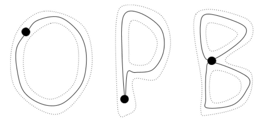
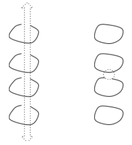
To describe a shape’s connectivity, you can count the number of “loops” in the shape, starting from an initial point called the basepoint. For example, the letters “O” and “P” are said to have the same connectivity because they each have one loop, whereas the letters “O” and “B” are said to have different connectivity because “O” has one loop and “B” has two loops. Algebraic topology takes this idea of classifying shapes based on how many loops they have, and extends it to spaces of arbitrarily many dimensions (Carlsson, 2009).

For example, let’s start off with a two-dimensional space, a plane. Immediately, we run into a problem we didn’t have with letters: we can draw infinitely many loops in this infinite sheet. How should we count them all?

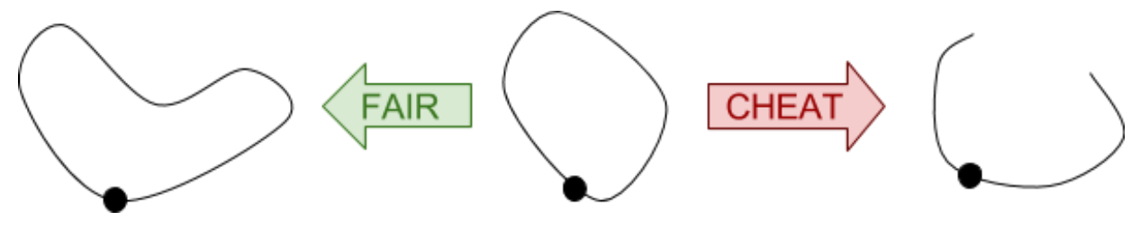
So that we’re not stuck counting loops for eternity, we say that loops are equivalent if they can be continuously deformed into each other. Given a loop, we can drag it across the plane, twist it around, stretch it, compress it, and so on, and it will still be the same loop. The only thing we aren’t allowed to do is tear it. That’s cheating.

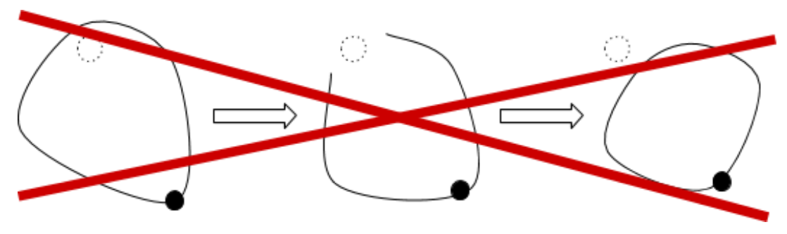
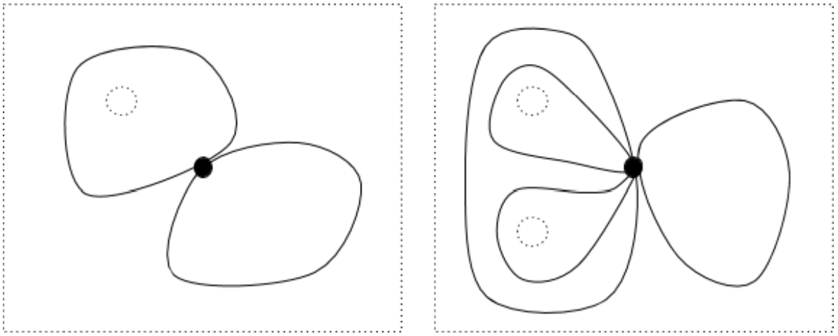
To count loops using this equivalence, we need to figure out how many distinct loops there are. In the plane above, it’s easy – there is only one distinct loop. However, if there is a hole in the sheet, the loop with the hole inside is not the same as the loop with the hole outside: if the hole is inside a loop, the only way to move it to the outside is to tear the loop, and that’s cheating.

A plane with one hole, then, has two loops: one loop with the hole inside and another loop with the hole outside. The loop with the hole inside can be deformed into any other loop with the hole inside, and the loop with the hole outside can be deformed into any other loop with the hole outside. For a plane with two holes, we have four distinct loops: one around each hole, one around both holes, and one around neither hole. Topologists have a word, homotopy, for the kind of non-tearing deformations we’re imagining, and they call the collection of distinct loops a homotopy group.

In higher-dimensional spaces, we need to count loops in each dimension. For example, consider a three-dimensional space with two points and a line removed. This looks like a cube of cheese that has two air bubbles and has been poked by a toothpick, infinitely enlarged.

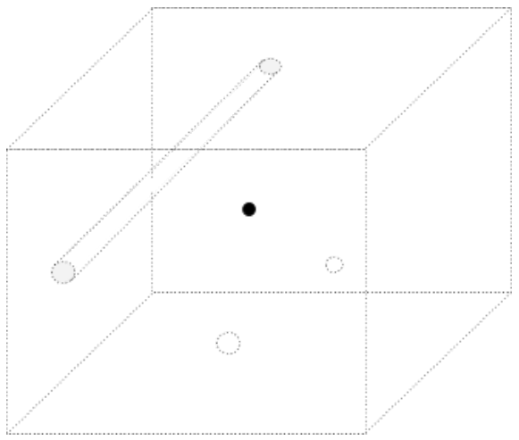
There are two one-dimensional loops: a circle with the line inside, and a circle with the line outside.

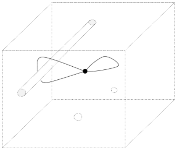
A circle containing the line is tethered to the line, but a circle containing the missing point can move above and below the point. Since circles can move through the missing points, the missing points do not affect the number of distinct one-dimensional loops.

There are four two-dimensional loops: a bubble with no points inside, a bubble with one point inside, a bubble with the other point inside, and a bubble with both points inside. The missing line does not affect the number of distinct two-dimensional loops because the line spans the entire space and consequently we cannot put the line inside of a bubble.

In higher dimensions, it’s helpful to think of loops as surfaces. A 1-dimensional loop (circle) is the surface of a 1-dimensional sphere (disk). A 2-dimensional loop (bubble) is the surface of a 2-dimensional sphere (solid sphere). In general, an n-dimensional loop is the surface of an n-dimensional sphere.

Approximating Topologies using Simplicial Complexes

Real-world datasets are not explicit topological spaces. Rather, they are collections of points sampled from topological spaces, and the goal of topological data analysis is to analyze these point clouds and infer information about their underlying topological spaces. One can do this by using the point cloud to construct a “simplicial complex” that approximates the underlying topological space (Carlsson, 2009).

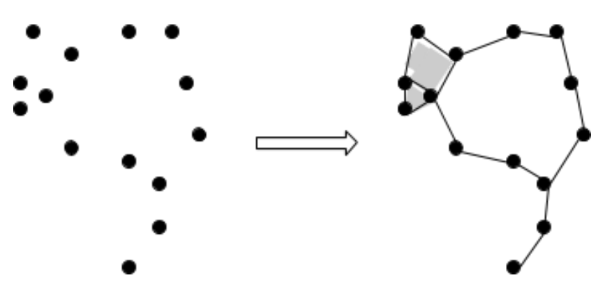
The main idea behind turning point clouds into simplicial complexes is to put epsilon-balls, or error margins, around points and use the overlaps to determine the connections in the simplicial complex. The constructions generated using different values of epsilon will correspond to topological approximations of the point cloud at different levels of scale.

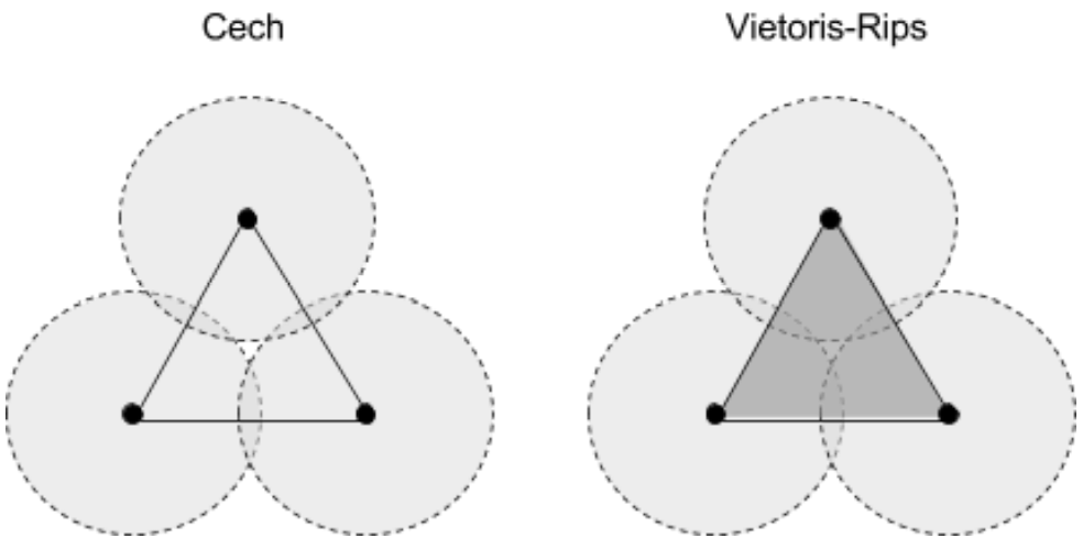
For example, one generates the Cech complex of a point cloud by adding an n-simplex whenever the intersection of all n balls is nonempty. A more computationally efficient method, which generates the Vietoris-Rips complex, adds an n-simplex whenever the intersection of every pair in the n balls is nonempty, and contains the Cech complex as a subcomplex.

To see how these complexes are constructed, first consider these three points with pairwise-overlapping balls.

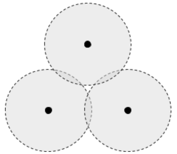
The associated Cech complex includes three points and three segments, but no triangle because the three balls don’t all overlap together anywhere. However, the Vietoris-Rips complex contains the triangle in addition to the three points and segments, since each pair of balls overlaps.

There is a theorem stating that for any epsilon, there is a finite set of points such that the Cech complex is homotopy-equivalent to the full space (this also applies to the Vietoris-Rips complex, since it contains the Cech complex). Therefore, in theory, our approximation should have the same topological features as the actual space, provided we use enough points.

Intuiting Homology in Topology

Unfortunately, homotopy groups are extremely difficult to compute in high dimensions. However, there is a similar concept, homology, that can be calculated on simplicial complexes via linear algebra (Carlsson, 2009). Like homotopy, homology also counts the number of loops of each dimension in a space, where loops are allowed to shift along the boundary of a higher-dimensional component on the space.

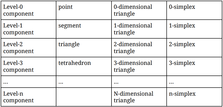
In simplicial complexes, the lowest-level components are points, followed by segments, and then triangles, and then solid tetrahedrons, and so on. You can think of an nth level component as an n-dimensional triangle, or more formally, an n-simplex.

For example, consider the following simplicial complex:

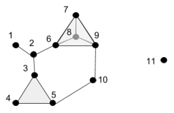
This complex contains the following simplices:

• 0-simplices: {1}, {2}, {3}, {4}, {5}, {6}, {7}, {8}, {9}, {10}, {11}
• 1-simplices: {1,2}, {2,3}, {2,6}, {3,4}, {3,5}, {4,5}, {5,10}, {6,7}, {6,8}, {6,9}, {7,8}, {7,9}, {8,9}, {9,10}
• 2-simplices: {3,4,5}, {6,7,8}, {6,7,9}, {6,8,9}, {7,8,9}

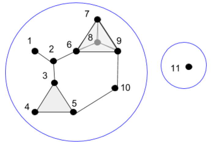
The 0th homology of this complex consists of those 0-dimensional loops along 0-simplices, which cannot be deformed into one another by shifting along the boundary of a 1-simplex. Put more simply, it consists of those points which cannot be shifted to one another along an edge. Since points {1} through {10} are all connected by paths through edges, they are all viewed as the same in first homology – but since {11} is not connected to any other point by an edge, it is different. Thus, the 0th homology of the above complex consists of two loops, which intuitively represent “point islands”: points {0} through {10} inhabit the first island, while point {11} is the lone inhabitant of the second island.

The 1st homology of this complex consists of those 1-dimensional loops along 1-simplices, which cannot be deformed into one another by shifting along the boundary of a 2-simplex. Put more simply, it consists of those edge loops which cannot be shifted to one another along triangles. For example, the two edge loops below are the same because {3,5} can be shifted to {3,4} and {4,5} on the triangle {3,4,5}, and {6,9} can be shifted to {6,7} and {7,9} on the triangle {6,7,9}.

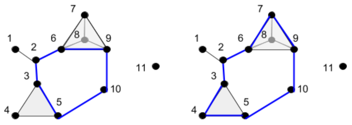
It turns out that, for this complex, there is no other edge loop that is different from the inner edge loop. Therefore, the 1st homology of the above complex consists of one loop, which intuitively represents the “donut hole” in the complex.

The 2nd homology is the last homology for this complex, because it contains no simplices beyond the 2nd dimension. It consists of those 2-dimensional loops along 2-simplices, which cannot be deformed into one another by shifting along the boundary of a 3-simplex. Put more simply, it consists of those closed (think “inflatable”) surfaces which cannot be stretched into to one another along solid tetrahedrons. The 2-simplices {3,4,5}, {6,7,8}, {6,7,9}, {6,8,9}, and {7,8,9} together form the surface of a tetrahedron, and the solid tetrahedron itself is not included in our complex. Therefore, the 2nd homology of the example complex consists of one loop, the surface of the tetrahedron.

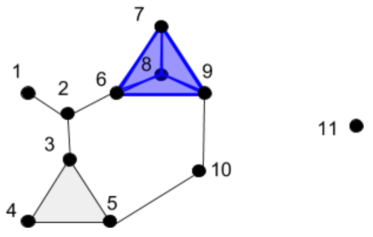
The number of components in the nth homology is called the nth Betti number, and by comparing the Betti numbers of different spaces, we can gain an idea of how topologically similar or different they are. For example, our complex had three nontrivial homologies, giving rise to Betti numbers (2, 1, 1). If we found two other datasets, constructed complexes on them, computed their homologies, and found that they had Betti numbers (2, 2, 1) and (1, 5, 3), then we would interpret the process generating the data of our example (2, 1, 1) complex as more similar to the process generating the data of the (2, 2, 1) complex, than the process generating the data of the (1, 5, 3) complex.

Measuring topological similarities between spaces by comparing their Betti numbers is just the tip of the iceberg. We have lots of mathematical machinery (e.g. probability and calculus) to analyze transformations between points, and Betti numbers give us a way to interpret entire spaces at points. This opens the door to studying not only relationships between parameters in a system, but also relationships between systems with completely different parameters.

Persistent Homology Barcodes

When we’re interested in topological features that persist across many scales of the data, we need consider all values of epsilon for the simplicial complex we construct on our data. This is the idea behind persistent homology: we can figure out which topological features persist over the full range of scale by making a plot that says whether a particular homology component was detected at some value of epsilon (Carlsson, 2009).

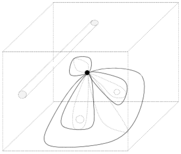
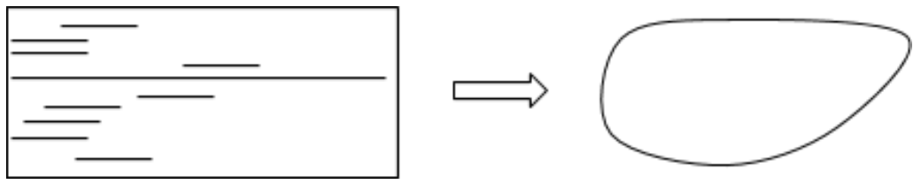
Barcode plots have values of epsilon on the horizontal axis, and a list of homology components on the vertical axis. Each row, then, corresponds to a homology component, and is shaded at values of epsilon where the homology component appears. For example, if the barcode plot below represents first homology, then a single long bar tells us that the dataset has a main loop that persists across many scales. Therefore, the dataset must look something like a circle.

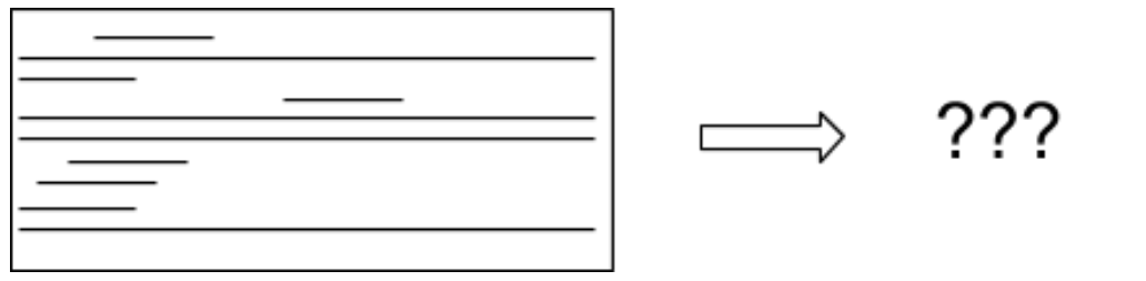
In a barcode plot with many long bars, many loops means many possibilities for the space. In these situations, we cannot always get a clear idea of what our space “looks” like, but we can still quantify the degree to which two datasets share the same topology by computing a similarity index between their persistence barcodes.

Persistence barcode distributions are currently an active area of research, and they can encode persistence of not only homology components, but also centrality, density, and other network measures.

References

1. Carlsson, Gunnar. "Topology and data." Bulletin of the American Mathematical Society 46.2 (2009): 255-308.

This post is part of the series The Data Scientist's Guide to Topological Data Analysis.

Want to get notified about new posts? Join the mailing list and follow on X/Twitter.