Intuiting Linear Regression
In linear regression, we model the target as a random variable whose expected value depends on a linear combination of the predictors (including a bias term).
This post is part of the series Intuiting Predictive Algorithms.
Want to get notified about new posts? Join the mailing list and follow on X/Twitter.
In linear regression, we model the target $y$ as a random variable whose expected value depends on a linear combination of the predictors $x$ (including a bias term, i.e. a column of 1s). When the noise is assumed to be Gaussian, MLE simplifies to least-squares:
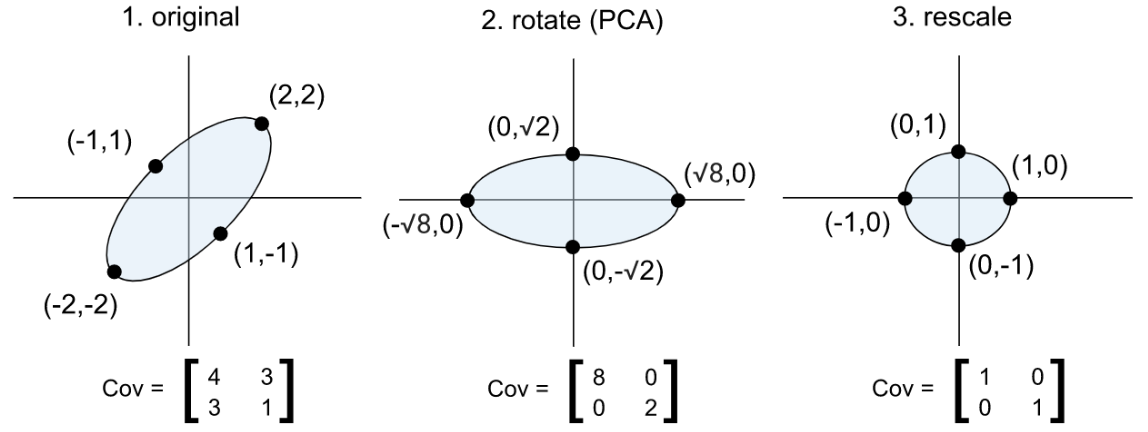
In multivariate linear regression, each $y_i$ is a vector containing multiple targets $y_{ij}.$ If the covariance matrix of the targets is a multiple of the identity matrix, then Gaussian MLE again simplifies to least squares. Provided the targets are linearly related, we can cause the covariance matrix to become a multiple of the identity matrix by converting the targets to an orthonormal basis of principal components (this is known as PCA, or principal component analysis).
One benefit of linear regression over more complex models is that linear regression is very interpretable. Provided the predictors are normalized and are not linearly dependent, the parameter or coefficient for a particular term can be interpreted as its “weight” in determining the prediction. Even if the predictors are linearly dependent, we can still make the model interpretable if we replace the predictors with a subset of their principal components before performing the regression. This is called Principal Component Regression.
Some other types of linear regression include polynomial, logistic, and regularized (ridge) regression. In polynomial regression, we include not just $x_i,$ but also $x_i^2,$ $x_i^3,$ etc. as predictors. In logistic regression, where the target is binary, we model the target as a Bernoulli random variable where the log of the odds ratio of the success probability is given by a linear regression:
In regularized or “ridge” regression, we assume a prior other than the Jeffreys prior. A Gaussian prior gives rise to L2 regularization:
A Laplacian prior gives rise to L1 regularization:
This post is part of the series Intuiting Predictive Algorithms.
Want to get notified about new posts? Join the mailing list and follow on X/Twitter.