Intuiting Maximum a Posteriori and Maximum Likelihood Estimation
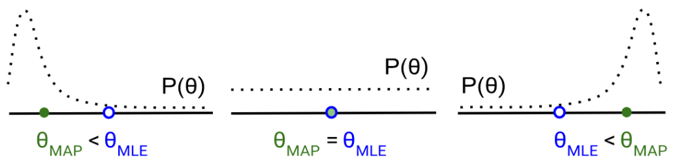
To visualize the relationship between the MAP and MLE estimations, one can imagine starting at the MLE estimation, and then obtaining the MAP estimation by drifting a bit towards higher density in the prior distribution.
This post is part of the series Intuiting Predictive Algorithms.
Want to get notified about new posts? Join the mailing list and follow on X/Twitter.
Given data $D = \lbrace ( (x_{ij}), y_i ) \rbrace,$ if we model the relationship between the predictors and the target as being governed by parameters $\theta = (\theta_i),$ then Bayes’ rule tells us that
We can interpret the integral as an average over all models, where the weight of a model’s contribution to the sum is governed by the $p(\theta \vert D)$ term. This term is called the posterior or “a posteriori” distribution, as it is the result of updating the prior or “a priori” distribution $p(\theta)$ (which reflects our previous beliefs about the parameters) with the information that the data tells us.
The average is difficult to compute, since the number of models grows exponentially with the number of parameters. It is easier to just pick the model with the maximum a priori distribution, rather than averaging over the entire ensemble. This is called Maximum A Posteriori (MAP) estimation.
If we want to model as though we know nothing aside from what the data tells us, then we can use the Jeffreys prior, which assigns $p(\theta)$ as a uniform distribution and is also known as the “uninformative” or “improper” prior since it does not actually depend on $\theta.$ When we perform MAP estimation using the Jeffreys prior, we are doing what is known as Maximum Likelihood Estimation (MLE). MLE derives its name from the fact that MAP with the Jeffreys prior amounts to maximizing $p(D \vert \theta),$ which is known as the likelihood.
To visualize the relationship between the MAP and MLE estimations, one can imagine starting at the MLE estimation, and then obtaining the MAP estimation by drifting a bit towards higher density in the prior distribution.
This post is part of the series Intuiting Predictive Algorithms.
Want to get notified about new posts? Join the mailing list and follow on X/Twitter.