Introduction to Neural Network Regressors

by Justin Skycak (@justinskycak) on February 05, 2022

The deeper or more "hierarchical" a computational graph is, the more complex the model that it represents.

This post is part of the book Introduction to Algorithms and Machine Learning: from Sorting to Strategic Agents. Suggested citation: Skycak, J. (2022). Introduction to Neural Network Regressors. In Introduction to Algorithms and Machine Learning: from Sorting to Strategic Agents. https://justinmath.com/introduction-to-neural-network-regressors/

Want to get notified about new posts? Join the mailing list and follow on X/Twitter.

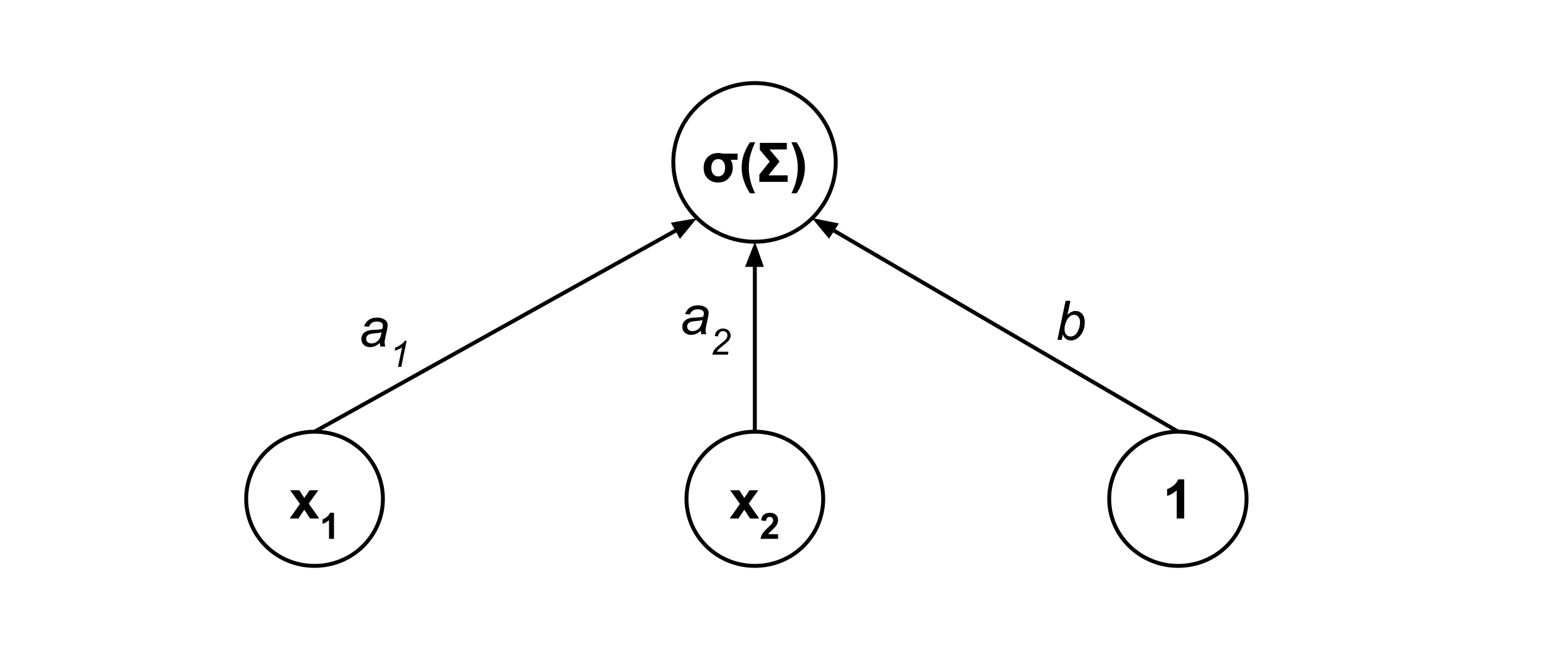
It’s common to represent models via computational graphs. For example, consider the following multiple logistic regression model:

$\begin{align*} f(x) &= \dfrac{1}{1 + e^{-(a_1 x_1 + a_2 x_2 + b)}} \end{align*}$

This model can be represented by the following computation graph, where

$\Sigma = a_1 x_1 + a_2 x_2 + b$ is the sum of products of lower-node values and the edge weights, and
$\sigma(\Sigma) = \dfrac{1}{1+e^{-\Sigma}}$ is the sigmoid function.

Hierarchy and Complexity

Loosely speaking, the deeper or more “hierarchical” a computational graph is, the more complex the model that it represents. For example, consider the computational graph below, which contains an extra “layer” of nodes.

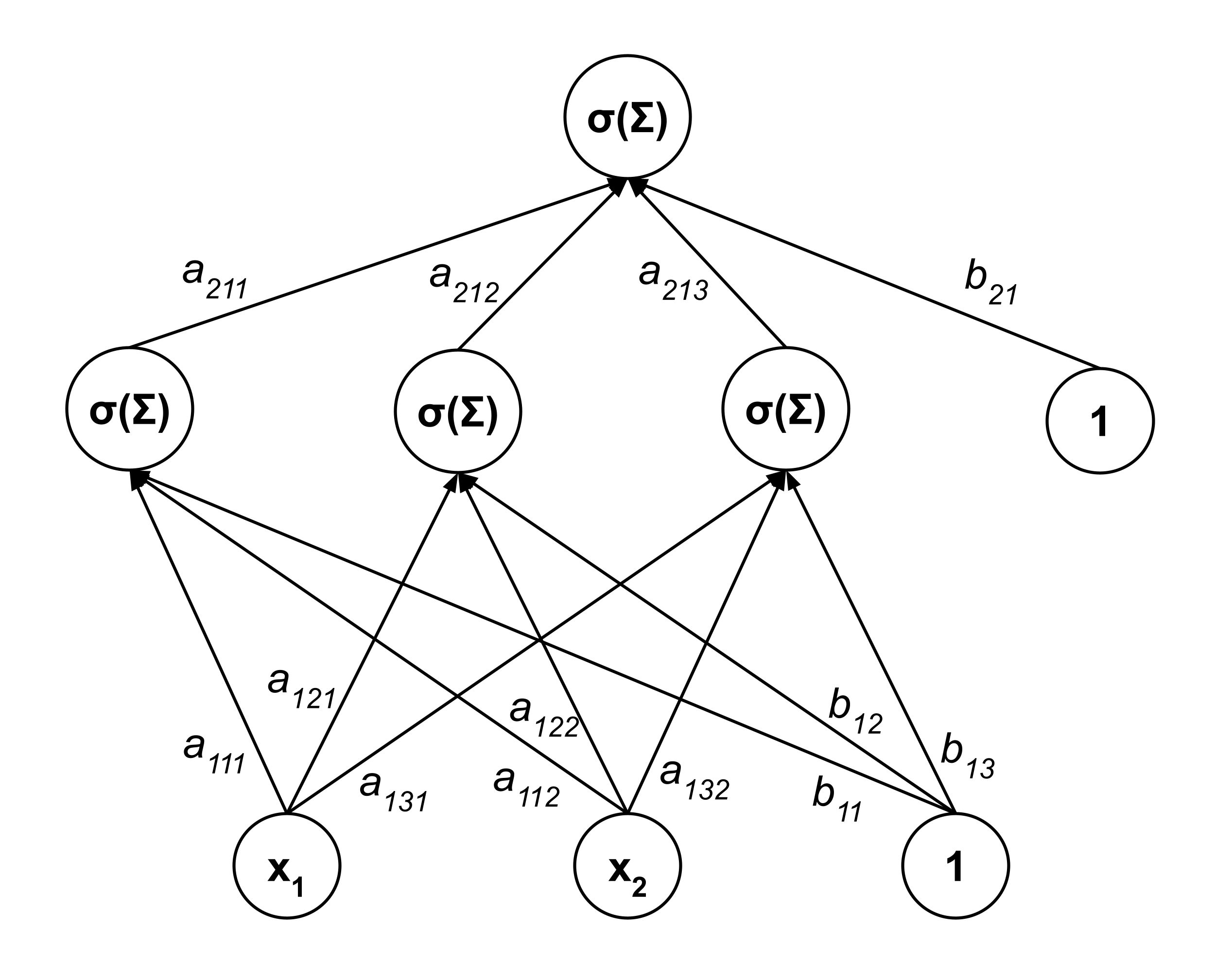
Whereas the first computational graph represented a simple model $f(x_1, x_2) = \sigma(a_1 x_1 + a_2 x_2 + b),$ this second computational graph represents a far more complex model:

$\begin{align*} f(x_1, x_2) &= \sigma \left( \begin{matrix} \phantom{+} a_{211} \sigma \left( a_{111} x_1 + a_{112} x_2 + b_{11} \right) \\ + a_{212} \sigma \left( a_{121} x_1 + a_{122} x_2 + b_{12} \right) \\ + a_{213} \sigma \left( a_{131} x_1 + a_{132} x_2 + b_{13} \right) \\ + b_{21\phantom{0}} \phantom{\sigma \left( a_{131} x_1 + a_{132} x_2 + b_{13} \right)} \end{matrix} \right) \end{align*}$

The subscripts in the coefficients may look a little crazy, but there is a consistent naming pattern:

$a_{\ell i j}$ is the weight of the connection from the $j$th node in the $\ell$th layer to the $i$th node in the next layer.
$b_{\ell i}$ is the weight of the connection from the bias node in the $\ell$th layer to the $i$th node in the next layer. (A bias node is a node whose output is always $1.$)

Neural Networks

A neural network is a type of computational graph that is loosely inspired by the human brain. Each neuron in the brain receives input electrical signals from other neurons that connect to it, and the amount of signal that a neuron sends outward to the neurons it connects to depends on the total amount of electrical signal it receives as input. Each connection has a different strength, meaning that neurons influence each other by different amounts. Additionally, neurons in key information-processing parts of the brain are sometimes arranged in layers.

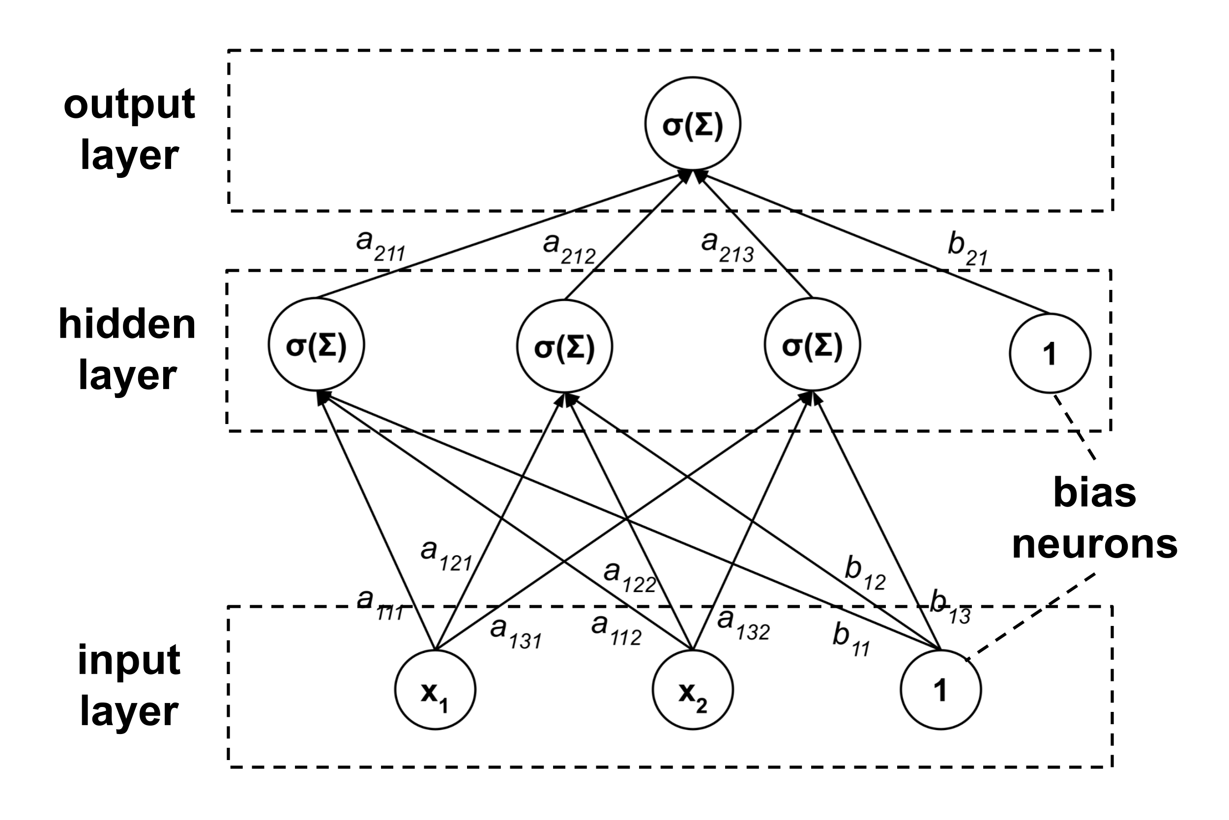
Using neural network terminology, the computational graph above can be described as a neural network with $3$ layers:

an input layer containing $2$ linearly-activated neurons and a bias neuron,
a hidden layer containing $3$ sigmoidally-activated neurons and a bias neuron, and
an output layer containing a single sigmoidally-activated neuron.

To say that a neuron is sigmoidally-activated means that to get the neuron’s output we apply a sigmoidal activation function $\sigma$ to the neuron’s input. Remember that the input $\Sigma$ is the sum of products of lower-node values and the edge weights. By convention, a linear activation function is the identity function (i.e. the output is the same as the input).

Neural networks are extremely powerful models. In fact, the universal approximation theorem states that given a continuous function $f: [0,1]^n \to [0,1]$ and an acceptable error threshold $\epsilon > 0,$ there exists a sigmoidally-activated neural network with one hidden layer containing a finite number of neurons such that the error between the $f$ and the neural network’s output is less than $\epsilon.$

Example: Manually Constructing a Neural Network

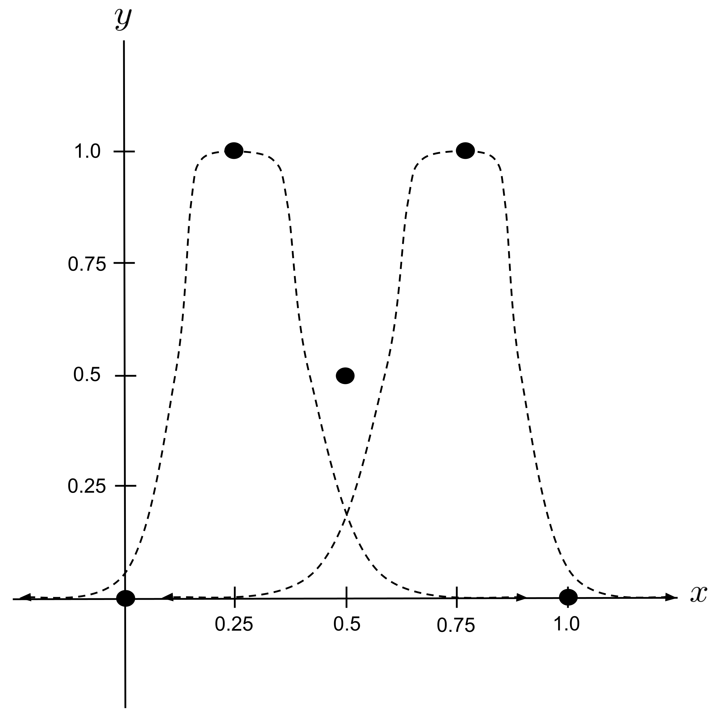
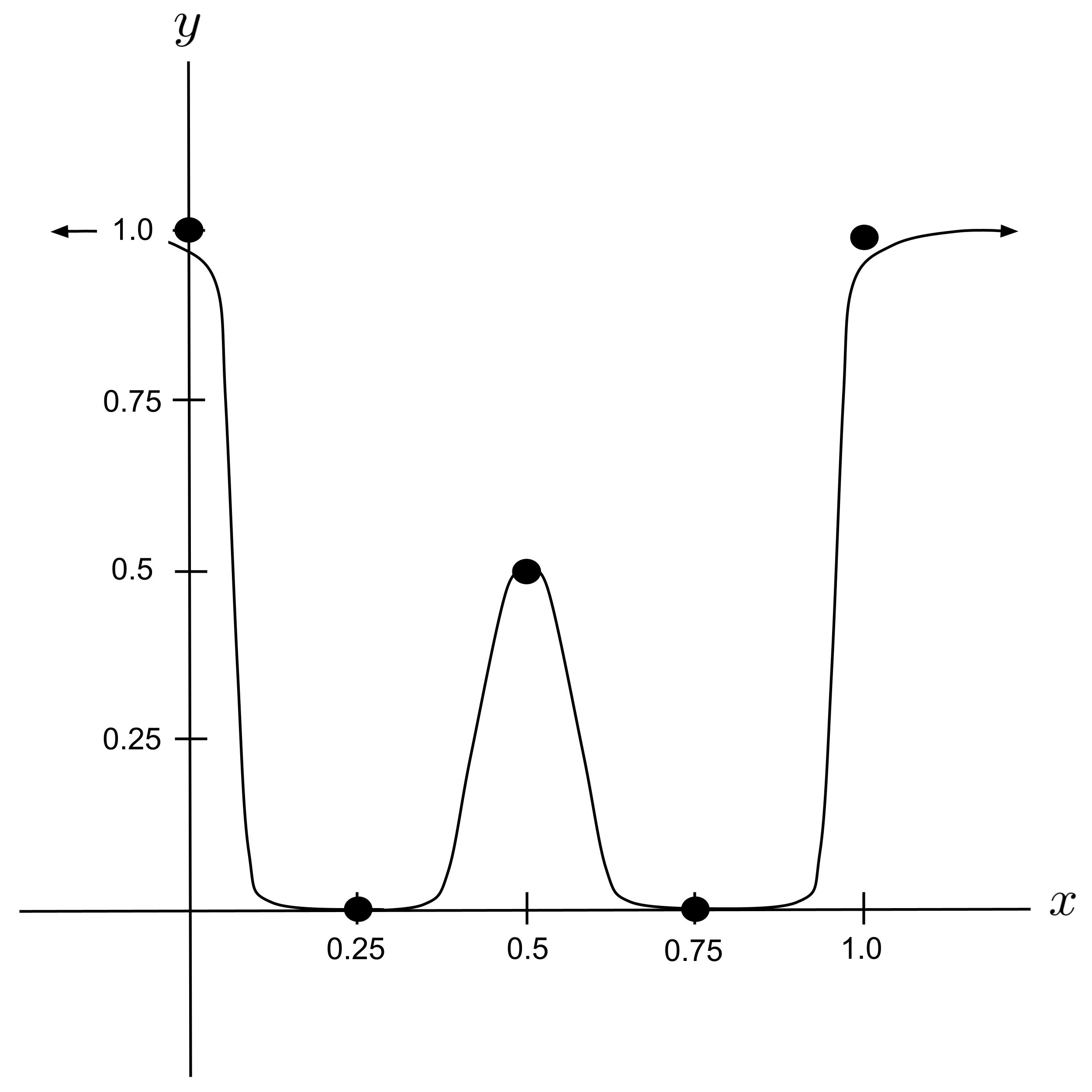
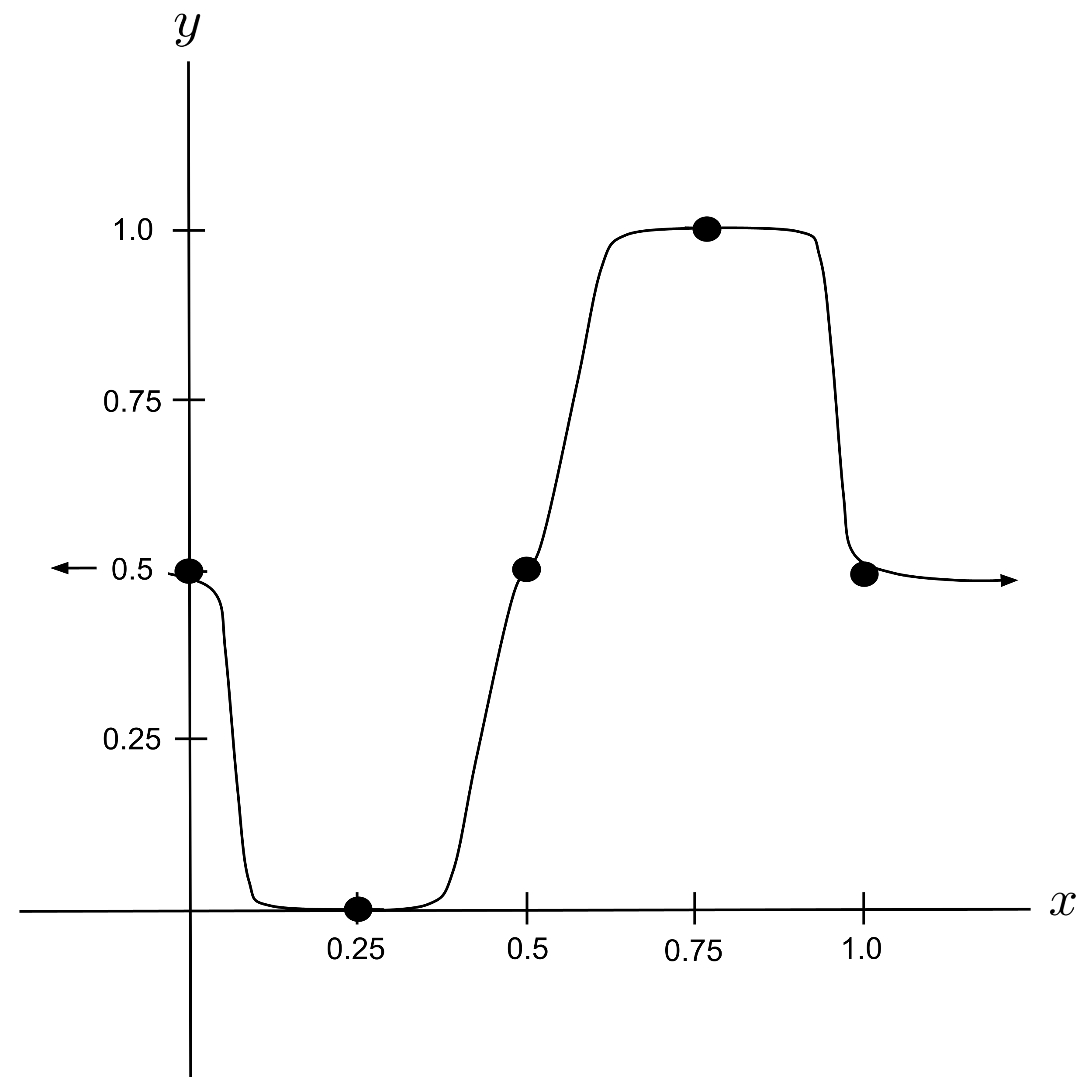
To demonstrate, let’s set up a neural network that models the following data set:

$\begin{align*} \left[ (0,0), (0.25,1), (0.5,0.5), (0.75,1), (1,0) \right] \end{align*}$

First, we’ll draw a curve that approximates the data set. Then, we’ll work backwards to combine sigmoid functions in a way that resembles the curve that we drew.

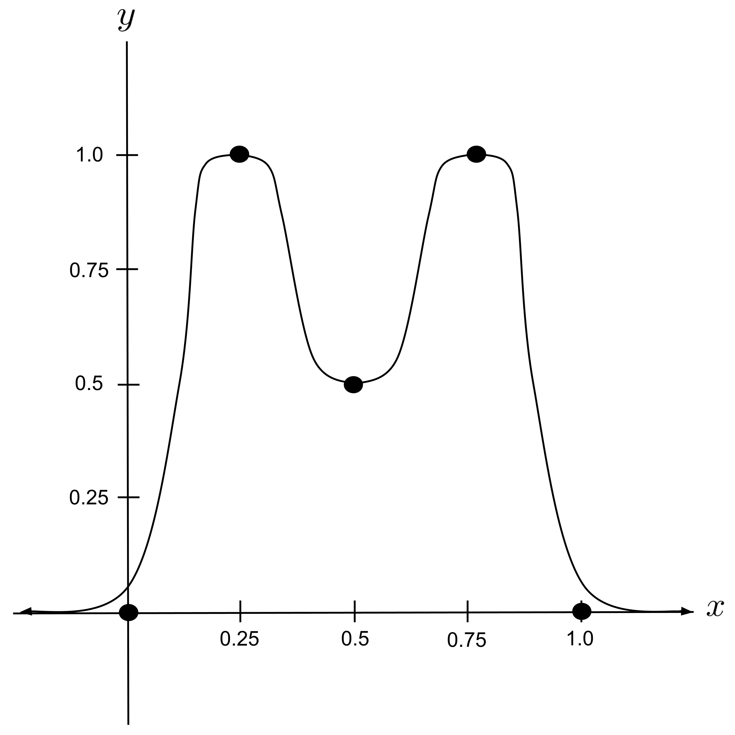
Loosely speaking, it appears that our curve can be modeled as the sum of two humps.

Notice that we can create a hump by adding two opposite-facing sigmoids (and shifting the result down to lie flat against the $x$-axis):

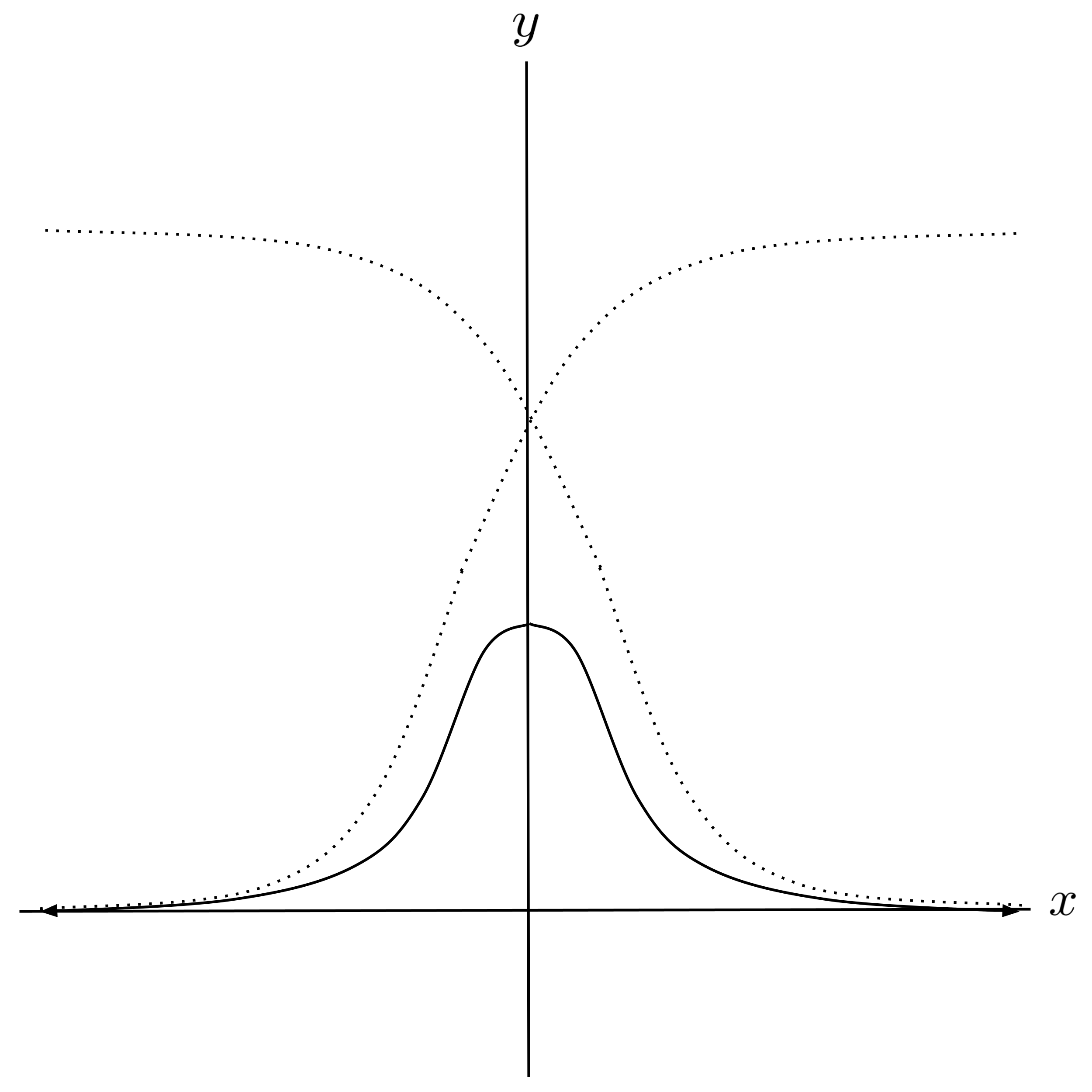
$\begin{align*} h(x) = \sigma(x+1) + \sigma(-x+1)-1 \end{align*}$

Remember that our neural network repeatedly applies sigmoid functions to sums of sigmoid functions, so we’ll have to apply a sigmoid to the function above. The following composition will accomplish this while shaping our hump to be the correct width:

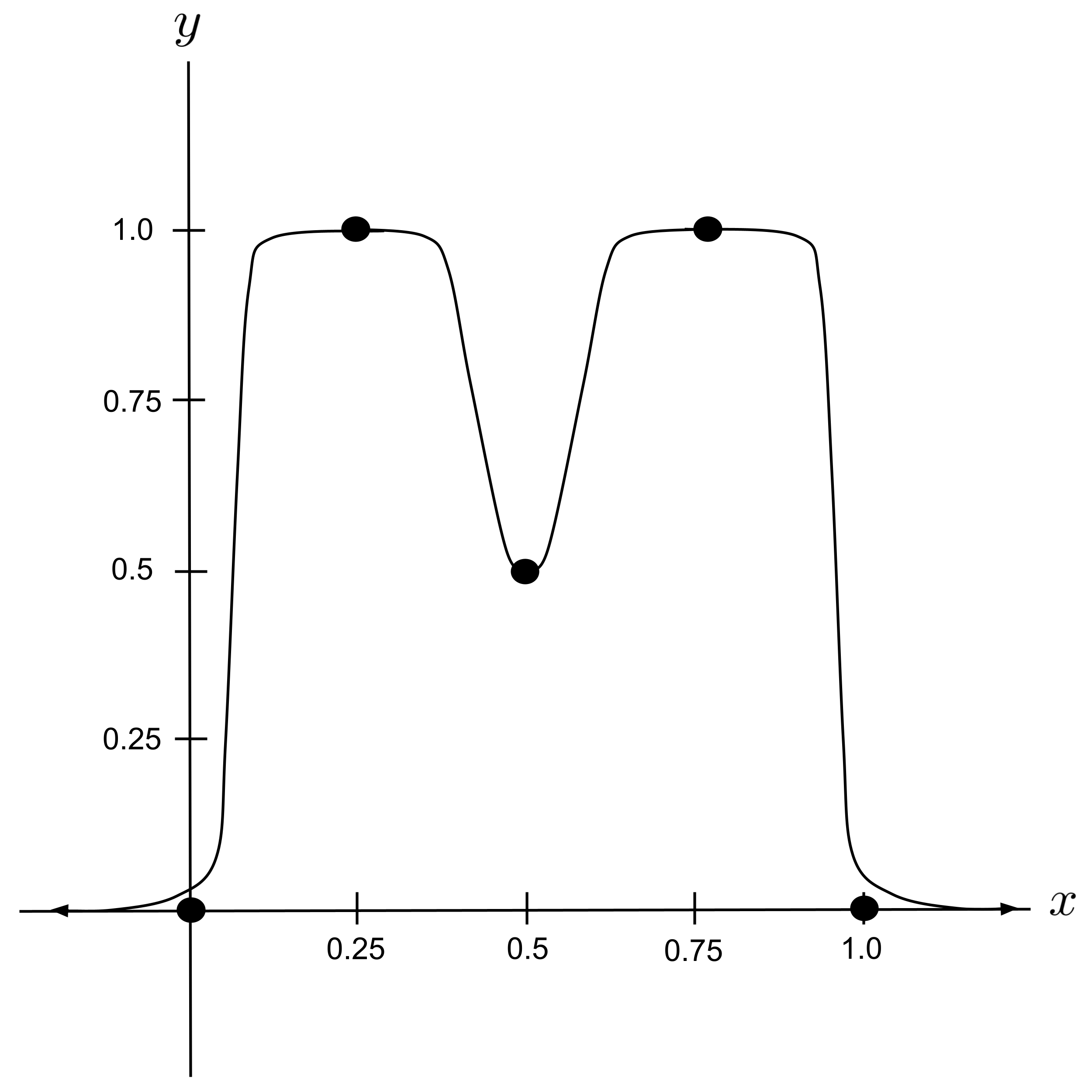
$\begin{align*} H(x) = \sigma( 20h(10x) - 5) \end{align*}$

Then, we can represent our final curve as the sum of two horizontally-shifted humps (again shifted downward to lie flat against the $x$ axis and then wrapped in another sigmoid function).

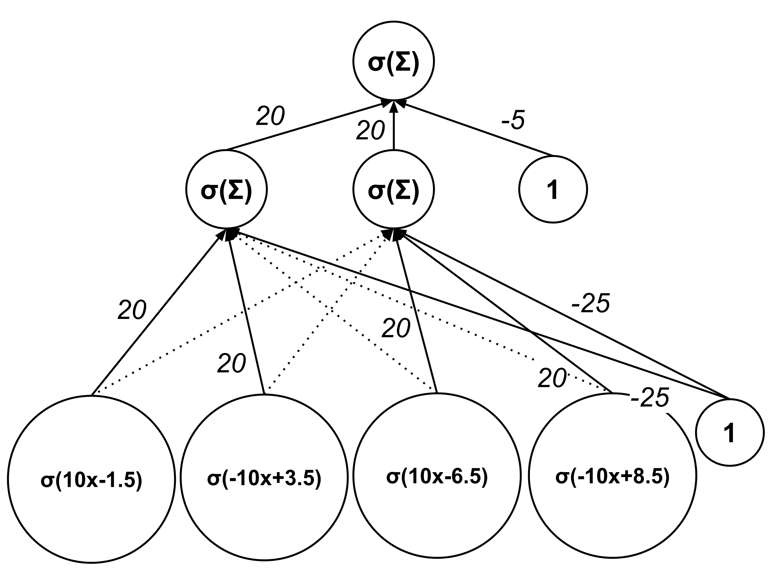
$\begin{align*} \sigma( 20 H(x-0.25) + 20H(x-0.75)-5 ) \end{align*}$

Now, let’s work backwards from our final curve expression to figure out the architecture of the corresponding neural network.

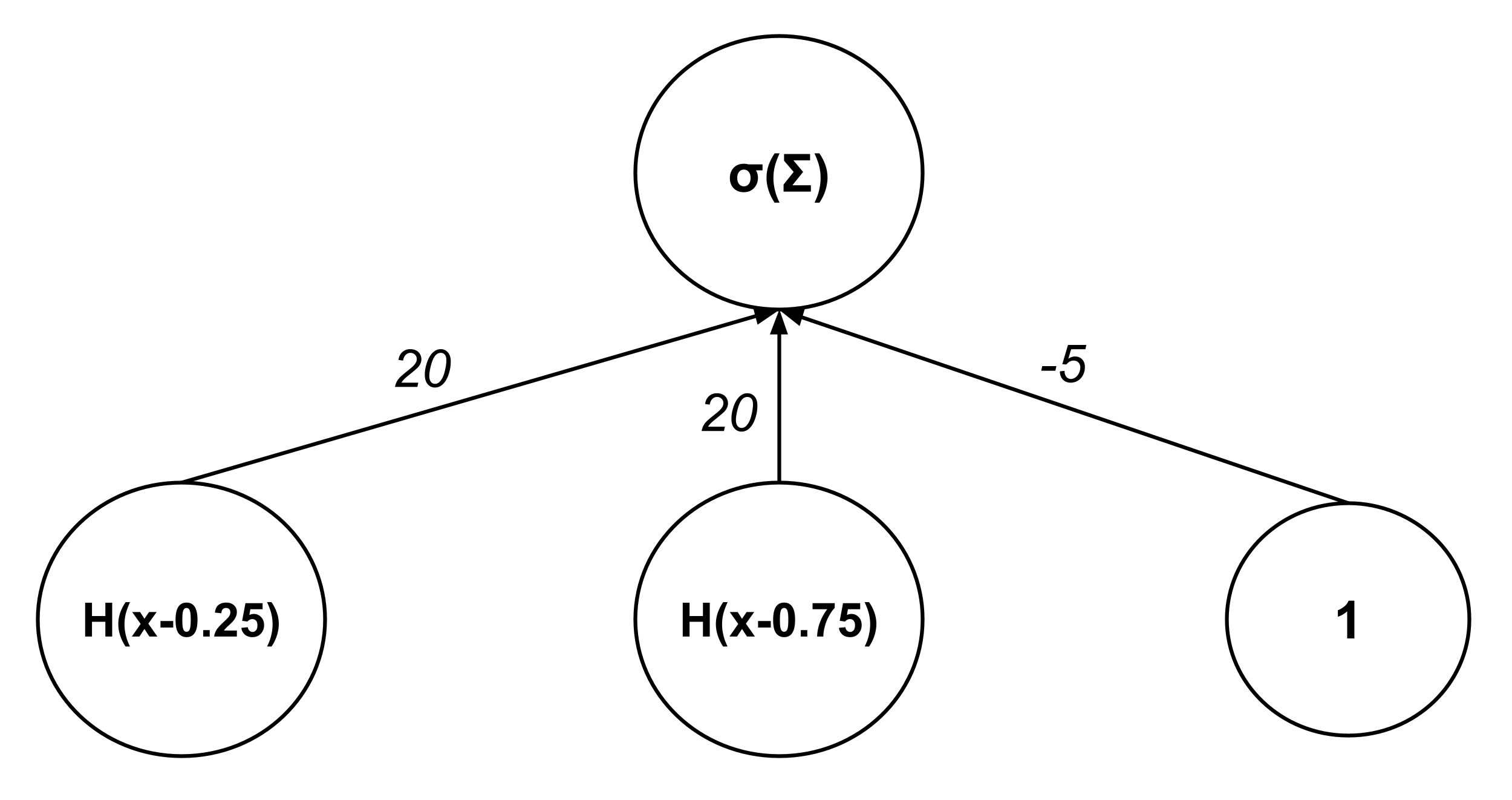
Our output node represents the expression

$\begin{align*} \sigma( 20 H(x-0.25) + 20H(x-0.75)-5 ), \end{align*}$

so the previous layer should have nodes whose outputs are $H(x-0.25),$ $H(x-0.75),$ and $1$ (the corresponding weights being $20,$ $20,$ and $-5$ respectively).

Expanding further, we have

$\begin{align*} H(x-0.25) &= \sigma(20h(10x-2.5)-5) \\[3pt] &= \sigma(20(\sigma(10x-1.5)+\sigma(-10x+3.5)-1)-5) \\[3pt] &= \sigma( 20 \sigma(10x-1.5)+20\sigma(-10x+3.5)-25 ) \\ \\ H(x-0.75) &= \sigma(20h(10x-7.5)-5) \\[3pt] &= \sigma(20(\sigma(10x-6.5)+\sigma(-10x+8.5)-1)-5) \\[3pt] &= \sigma( 20 \sigma(10x-6.5)+20\sigma(-10x+8.5)-25 ), \end{align*}$

so the second-previous layer should have nodes whose outputs are $\sigma(10x-1.5),$ $\sigma(10x-6.5),$ $\sigma(-10x+3.5),$ $\sigma(-10x+8.5),$ and $1.$ (In the diagram below, edges with weight $0$ are represented by soft dashed segments.)

We can now sketch our full neural network as follows:

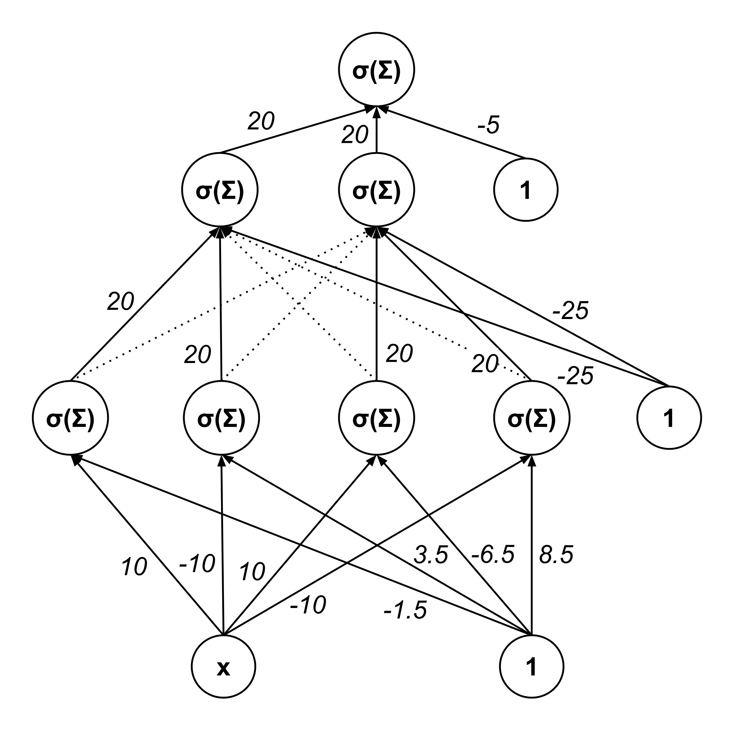
Hierarchical Representation

There is a clear hierarchical structure to the network. The first hidden layer transforms the linear intput into sigmoidal functions. The second hidden layer combines those sigmoids to generate humps. The output layer combines humps into the desired output.

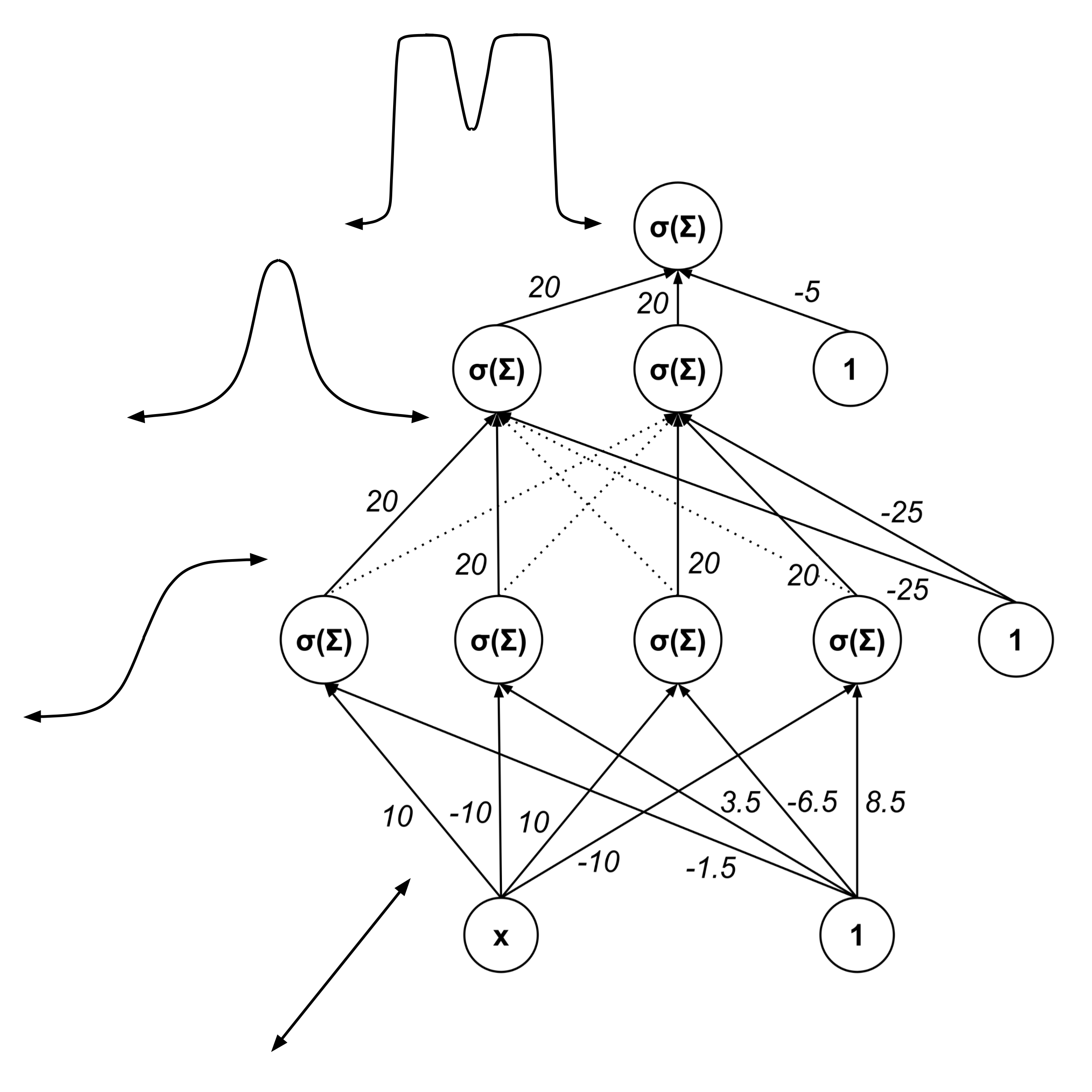
Hierarchical structure is ultimately the reason why neural networks can fit arbitrary functions to such high degrees of accuracy. Loosely speaking, each neuron in the network recognizes a different feature in the data, and deeper layers in the network synthesize elementary features into more complex features.

Exercises

Reproduce the example above by plotting the regression curve (as well as the data points).
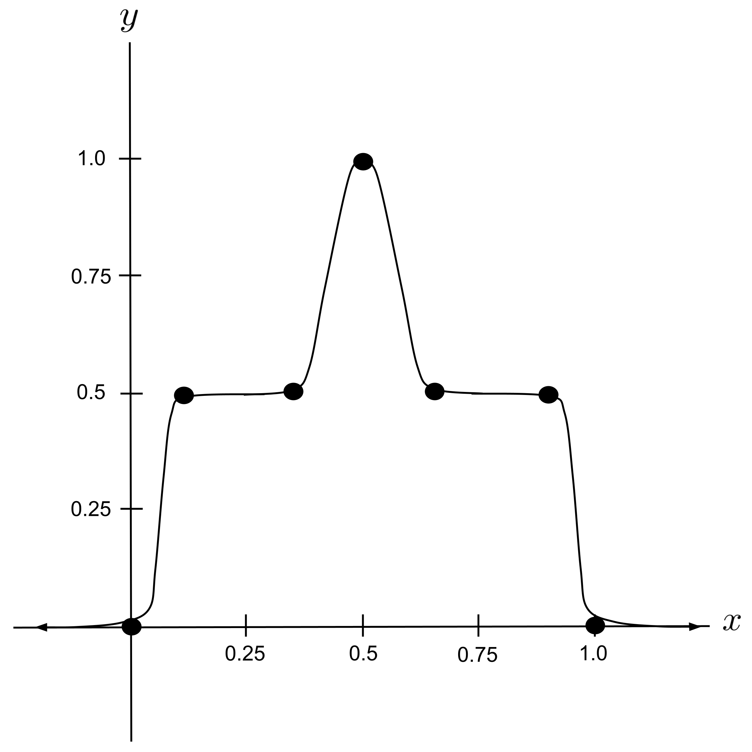
Tweak the neural network constructed in the discussion above so that the output resembles the following curve:
Tweak the neural network constructed in the discussion above so that the output resembles the following curve. (Hint: shift the equilibrium, flip one of the humps, and make the humps a little narrower.)
Tweak the neural network constructed in the discussion above so that the output resembles the following curve. (Hint: put a sharp peak on top of a wide plateau.)

Want to get notified about new posts? Join the mailing list and follow on X/Twitter.