Decision Trees

We can algorithmically build classifiers that use a sequence of nested "if-then" decision rules.

This post is a chapter in the book Introduction to Algorithms and Machine Learning: from Sorting to Strategic Agents. Suggested citation: Skycak, J. (2022). Decision Trees. Introduction to Algorithms and Machine Learning: from Sorting to Strategic Agents. https://justinmath.com/decision-trees/

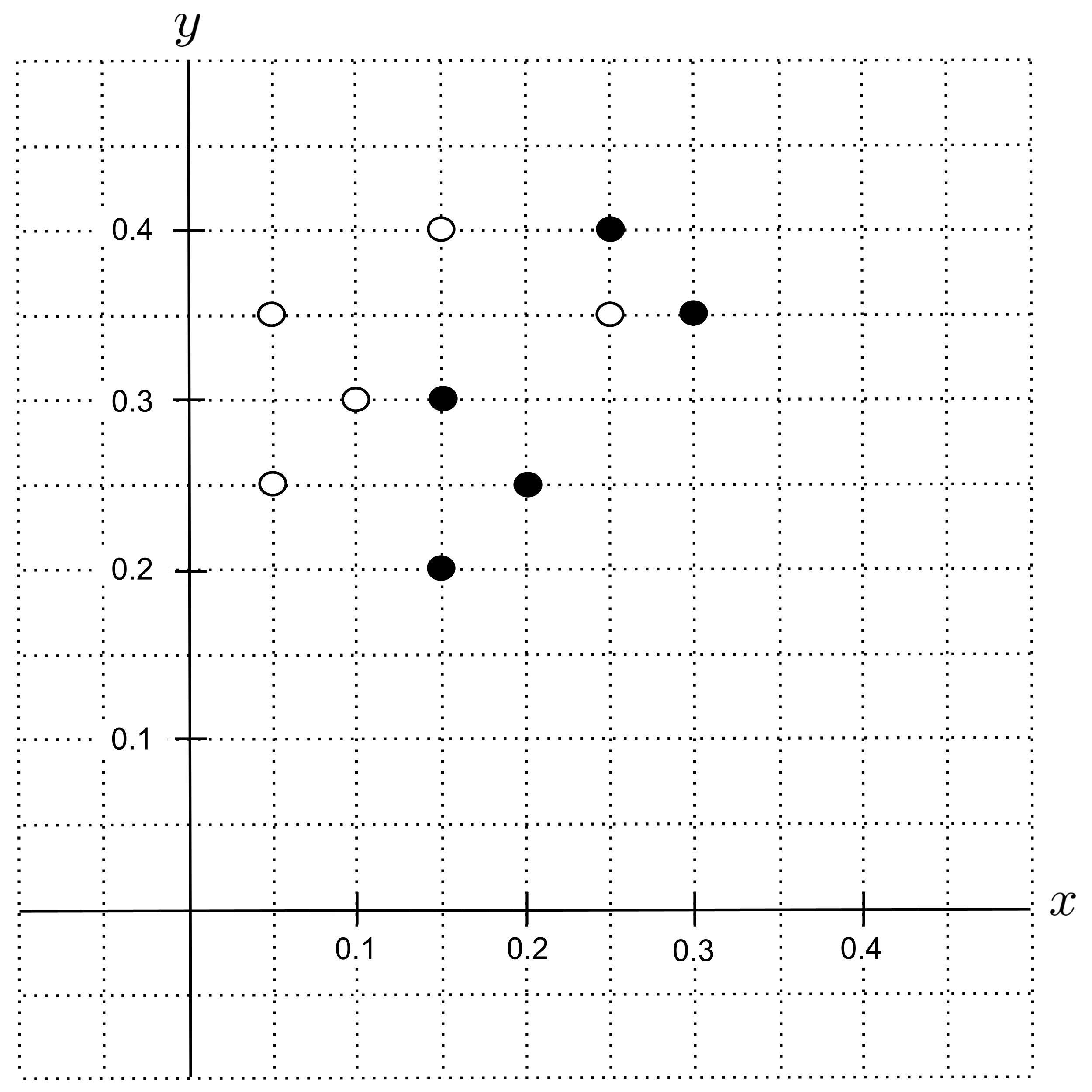
A decision tree is a graphical flowchart that represents a sequence of nested “if-then” decision rules. To illustrate, first recall the following cookie data set that was introduced during the discussion of k-nearest neighbors:

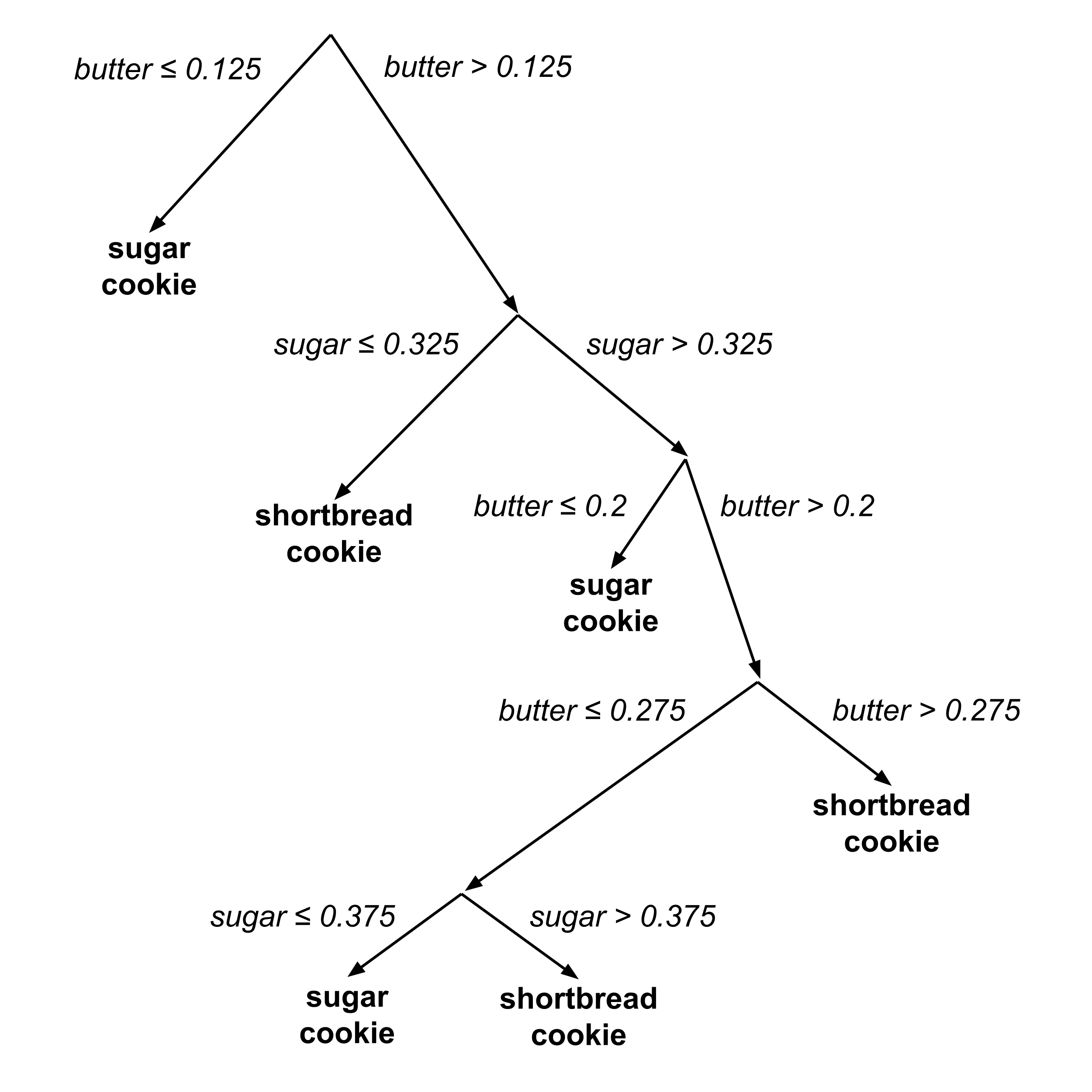
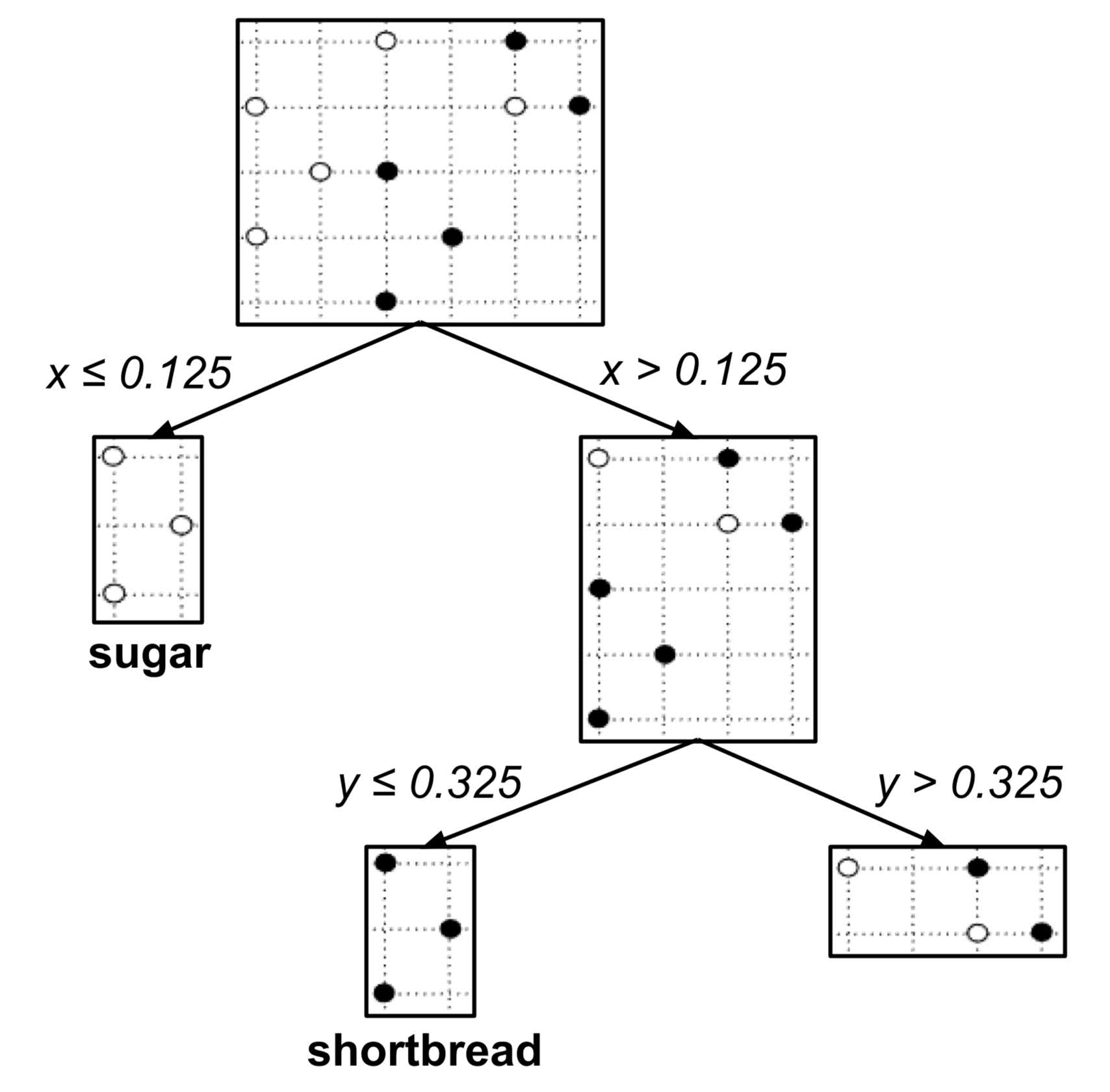
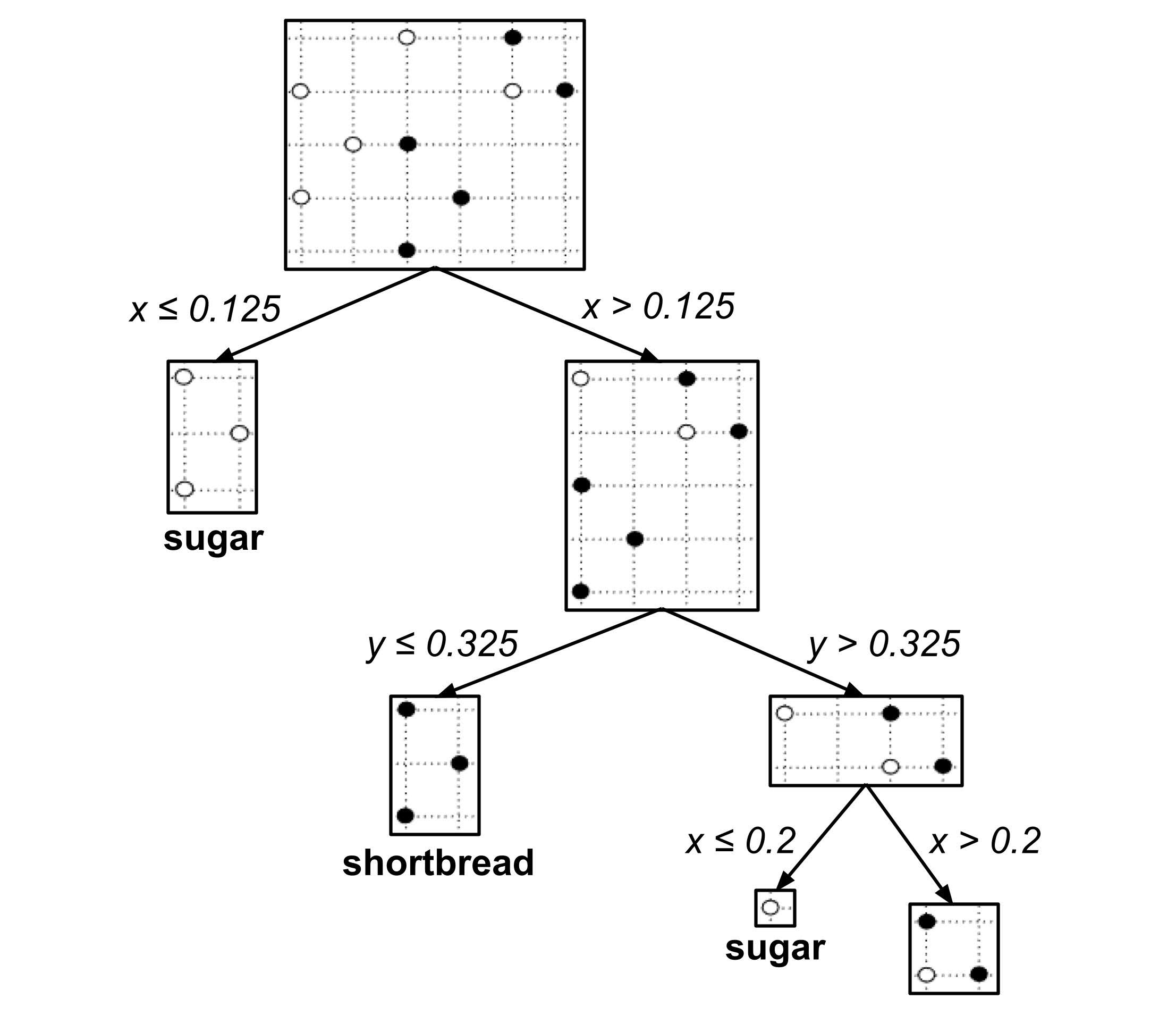
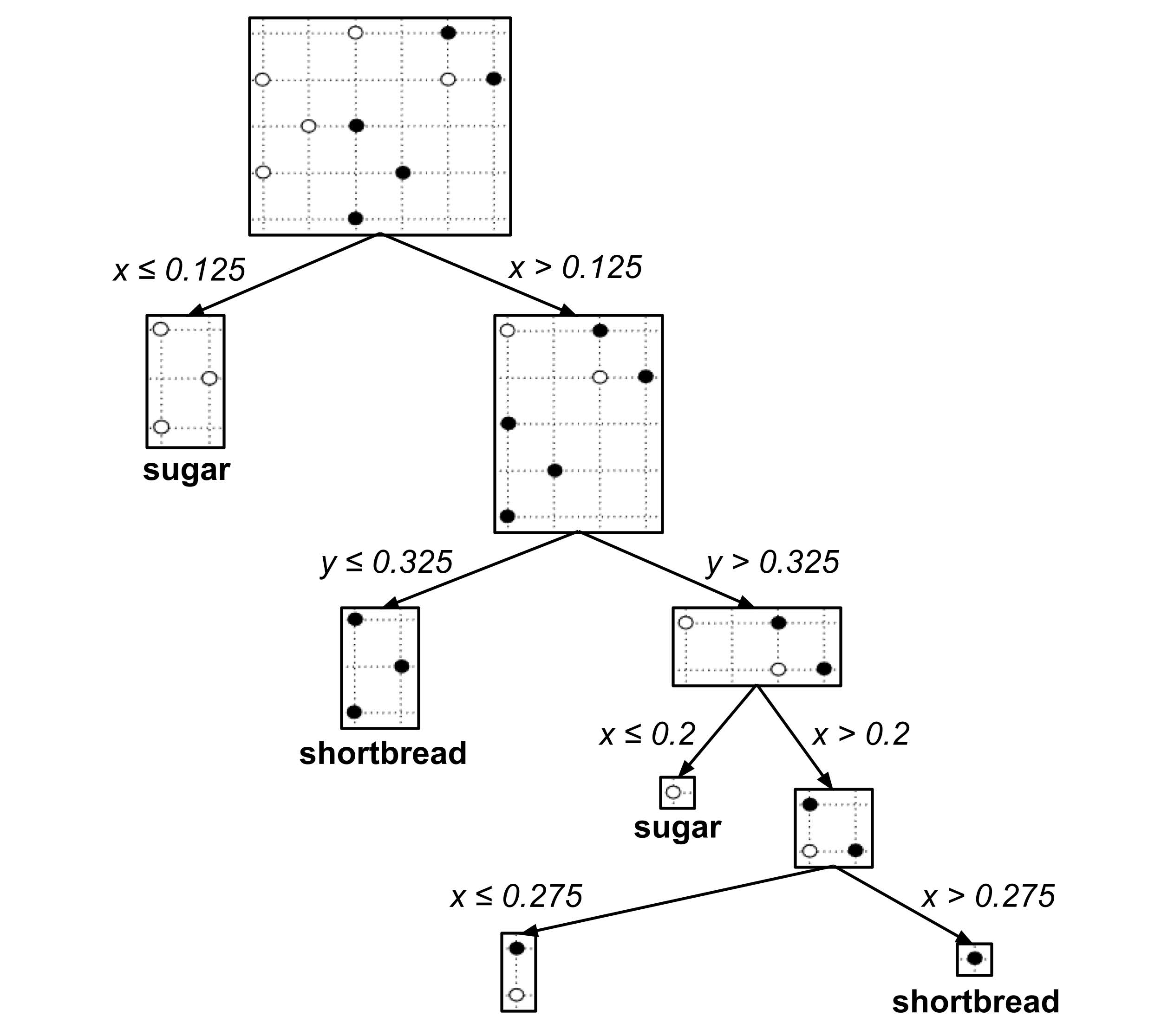
The following decision tree was algorithmically constructed to classify an unknown cookie as a shortbread cookie or sugar cookie based on its portions of butter and sugar.

Using a Decision Tree

To use the decision tree to classify an unknown cookie, we start at the top of the tree and then repeatedly go downwards and left or right depending on the values of $x$ and $y.$

For example, suppose we have a cookie with $0.25$ portion butter and $0.35$ portion sugar. To classify this cookie, we start at the top of the tree and then go

1. right $(\textrm{butter} > 0.125),$
2. right $(\textrm{sugar} > 0.325),$
3. right $(\textrm{butter} > 0.2),$
4. left $(\textrm{butter} \leq 0.275),$
5. left $(\textrm{sugar} \leq 0.375),$

reaching the prediction that the cookie is a sugar cookie.

Classification Boundary

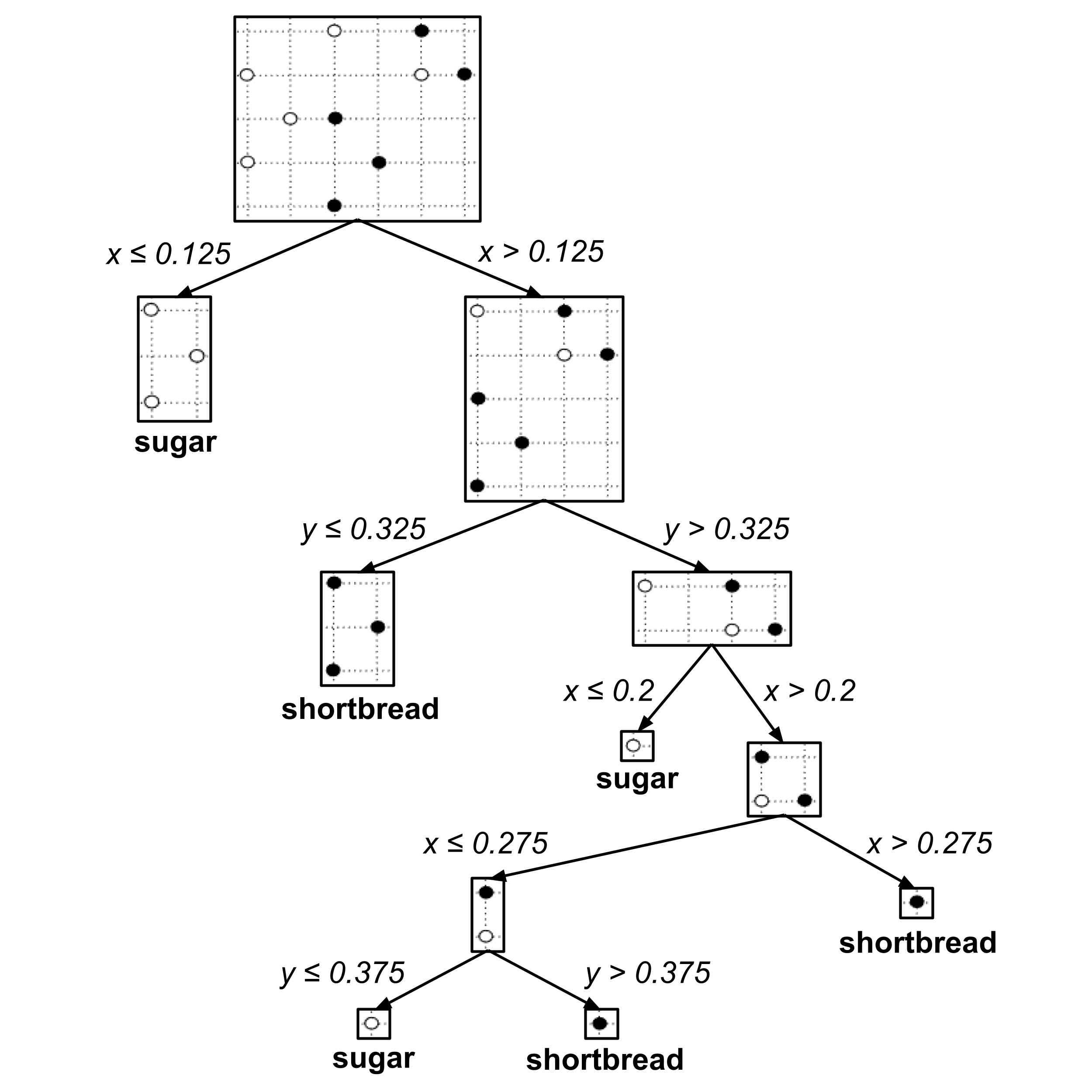
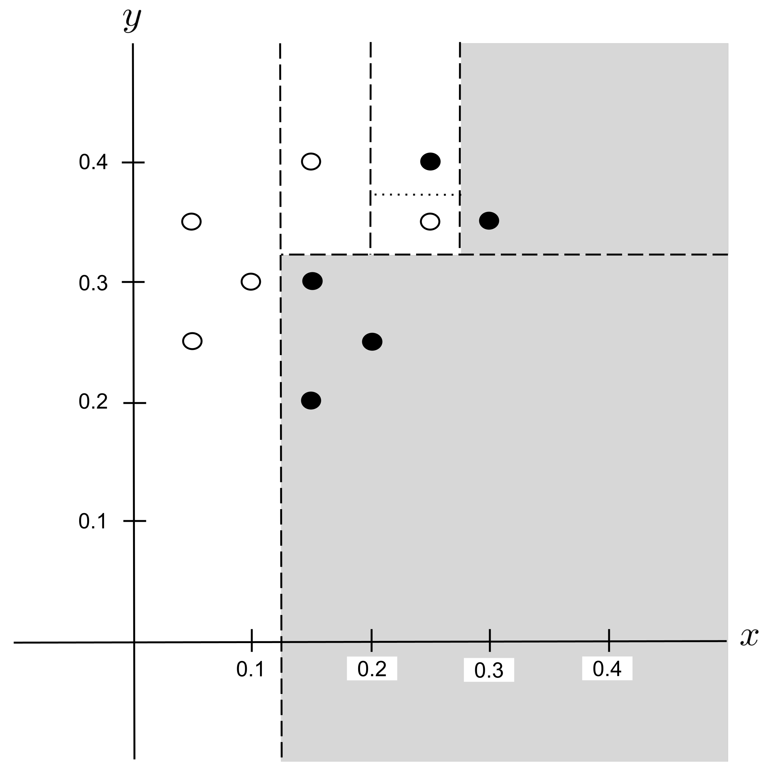
Let’s take a look at how the decision tree classifies the points in our data set:

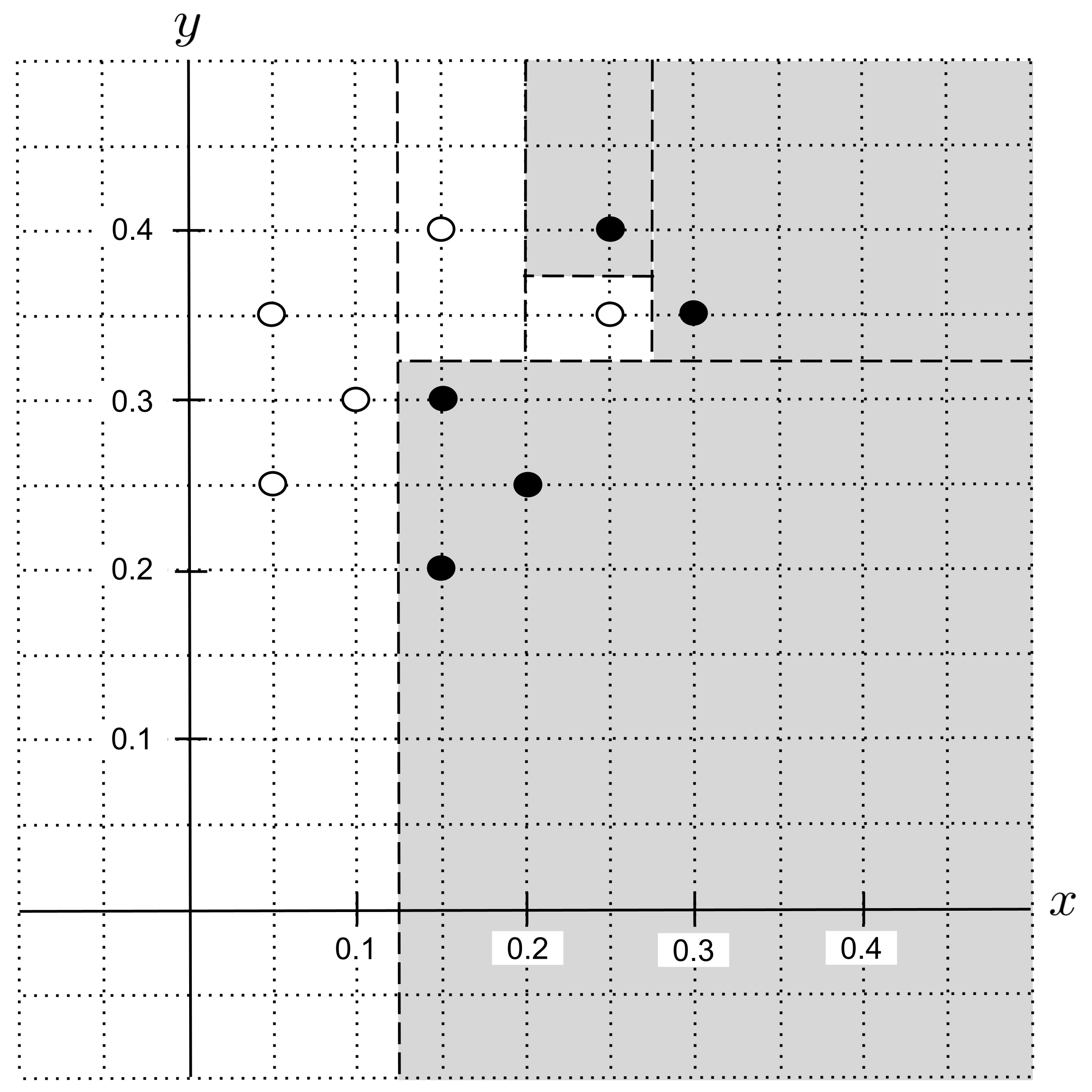
We can visualize this in the plane by drawing the classification boundary, shading the regions whose points would be classified as shortbread cookies and keeping unshaded the regions whose points would be classified as sugar cookies. Each dotted line corresponds to a split in the tree.

Building a Decision Tree: Reducing Impurity

The algorithm for building a decision tree is conceptually simple. The goal is to make the simplest tree such that the leaf nodes pure in the sense that they only contain data points from one class. So, we repeatedly split impure leaf nodes in the way that most quickly reduces the impurity.

Intuitively, a node has $0$ impurity when all of its data points come from one class. On the other hand, a node has maximum impurity when an equal amount of its data points come from each class.

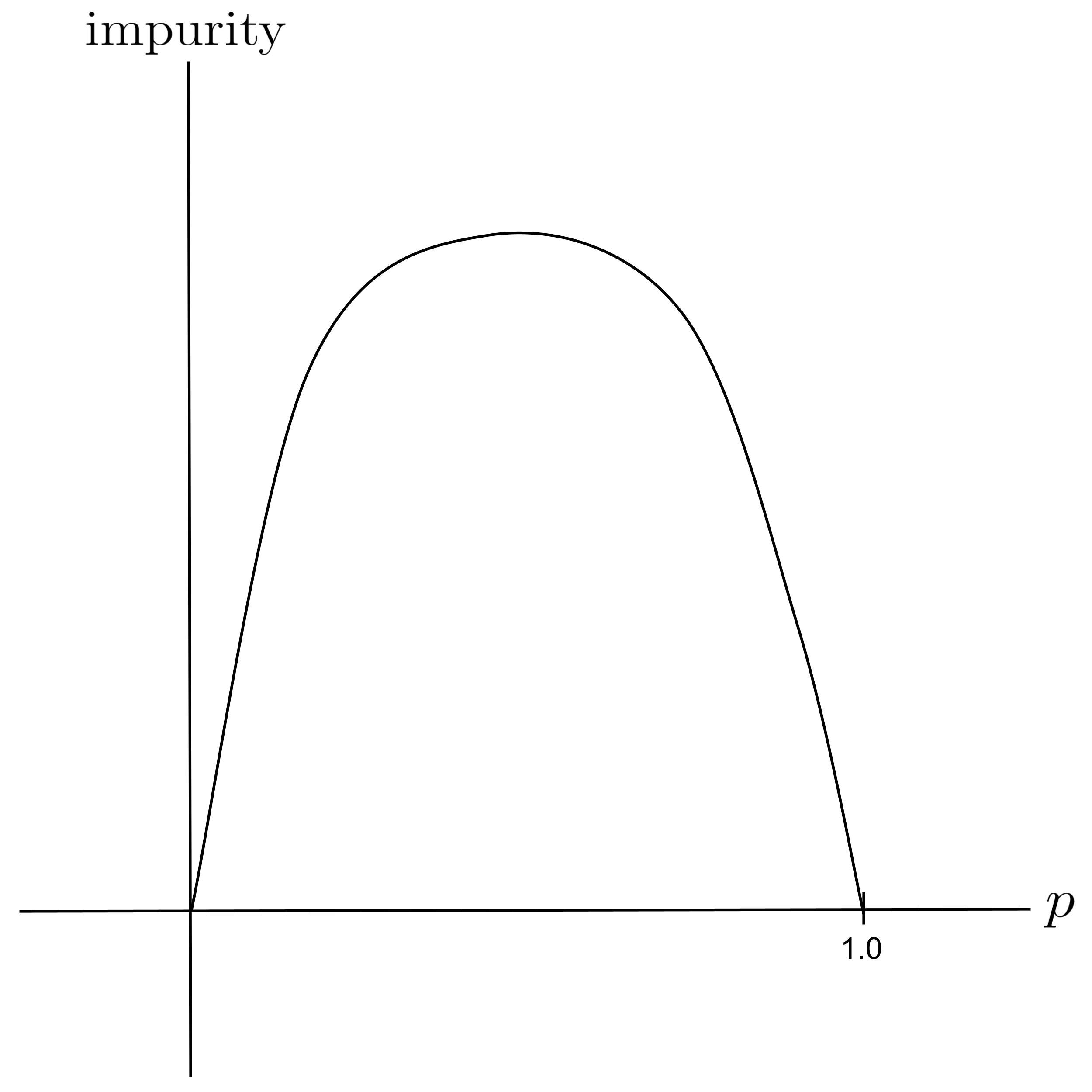
To quantify a node’s impurity, all we have to do is count up the proportion $p$ of the node’s data points that are from one particular class and then apply a function that transforms $p$ into a measure of impurity.

• If $p=0$ or $p=1,$ then the node has no impurity since its data points are entirely from one class.
• If $p=0.5,$ then the node has maximum impurity since half of its data points come from one class and the other half comes from the other class.

Graphically, our function should look like this:

Two commonly used functions that yield the above graph are Gini impurity, defined as

and information entropy, defined as

Although these functions may initially look a little complicated, note that their forms permit them to be easily generalized to situations where we have more than two classes:

where $p_i$ is the proportion of the $i$th class. (In our situation we only have two classes with proportions $p_1 = p$ and $p_2 = 1 - p.$)

Worked Example: Split 0

As we walk through the algorithm for building our decision tree, we’ll use Gini impurity since it simplifies nicely in the case of two classes, making it more amenable to manual computation:

Initially, our decision tree is just a single root node, i.e. a “stump” with no splits. It contains our full data set, shown below.

Worked Example: Split 1

Remember that our goal is to repeatedly split impure leaf nodes in the way that most quickly reduces the impurity. To find the split that most quickly reduces the impurity, we loop over all possible splits and compare the impurity before the split to the impurity after the split.

The impurity before the split is the same for all possible splits, so we will calculate it first. In the graph above there are $5$ points that represent shortbread cookies and $5$ points that represent sugar cookies, so $p=\dfrac{5}{5+5}=\dfrac{1}{2}$ and the impurity is computed as

Now, let’s find all the possible splits. To find the values of $x$ that could be chosen for splits, we first find all the distinct values of $x$ that are hit by points and put them in order:

The possible splits along the $x$-axis are the midpoints between consecutive entries in the list above:

Performing the same process for $y$-coordinates, we get the following:

Let’s go through each possible split and measure the impurity after the split. In general, the impurity after the split is measured as a weighted average of the new leaf nodes resulting from the split:

The formula above can be represented more concisely as

Possible Split: $x_\textrm{split} = 0.075$

The $x \leq 0.05$ node would be pure with $2$ sugar cookies, giving an impurity of

On the other hand, the $x > 0.05$ node would contain $5$ shortbread cookies and $3$ sugar cookies, giving an impurity of

The $\leq$ node would contain $2$ points while the $>$ node would contain $8$ points, giving proportions $p_\leq = \dfrac{2}{10}$ and $p_> = \dfrac{8}{10}.$

Finally, the impurity after the split would be

Possible Split: $x_\textrm{split} = 0.125$

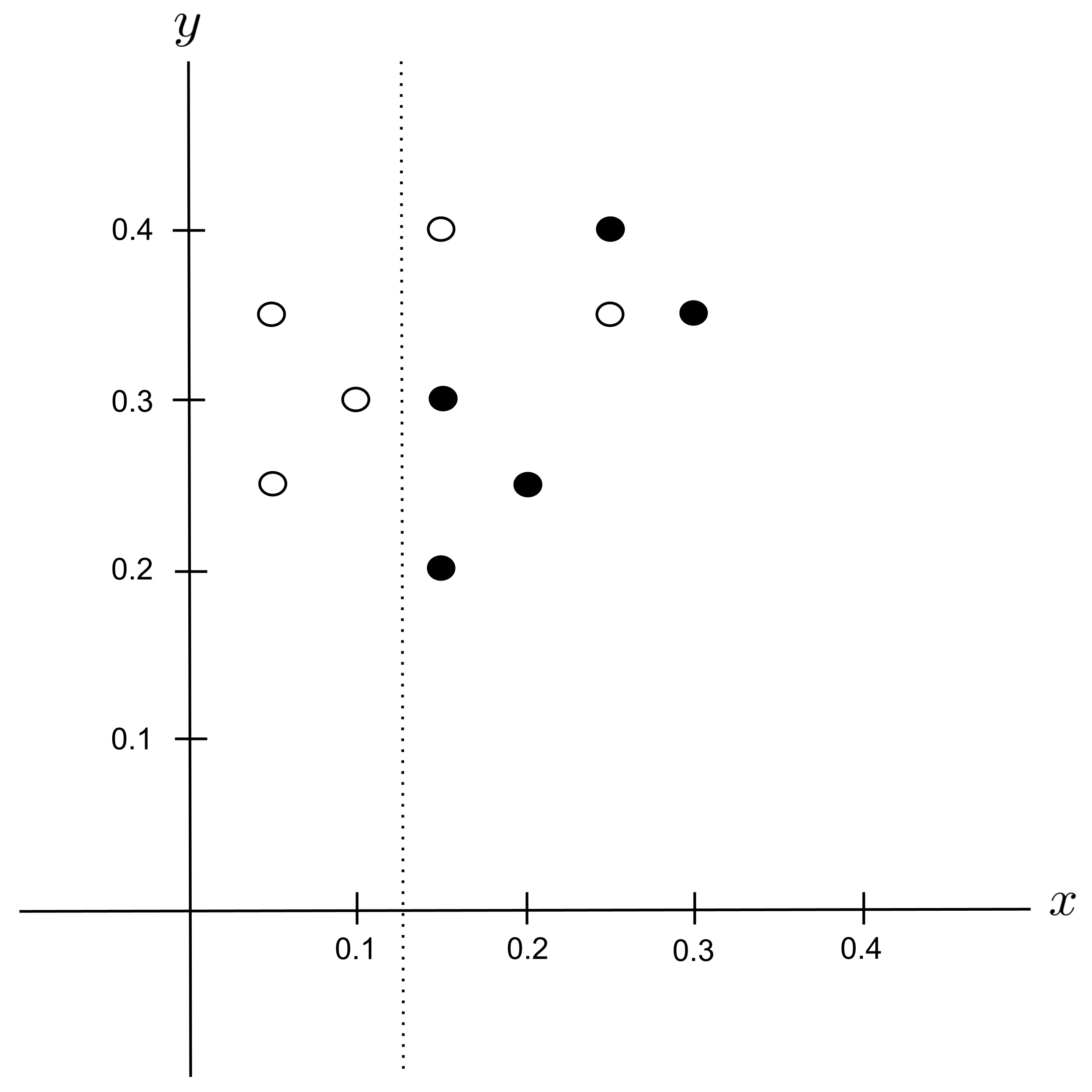
Repeating the same process, we have $p_\leq = \dfrac{3}{10}$ and $p_> = \dfrac{7}{10}$ get we get the following impurities:

Possible Split: $x_\textrm{split} = 0.175$

Possible Split: $x_\textrm{split} = 0.225$

Possible Split: $x_\textrm{split} = 0.275$

Possible Split: $y_\textrm{split} = 0.225$

Possible Split: $y_\textrm{split} = 0.275$

Possible Split: $y_\textrm{split} = 0.325$

Possible Split: $y_\textrm{split} = 0.375$

Best Split

Remember that the initial impurity before splitting was $G_\textrm{before} = 0.5.$ Let’s compute how much each potential split would decrease the impurity:

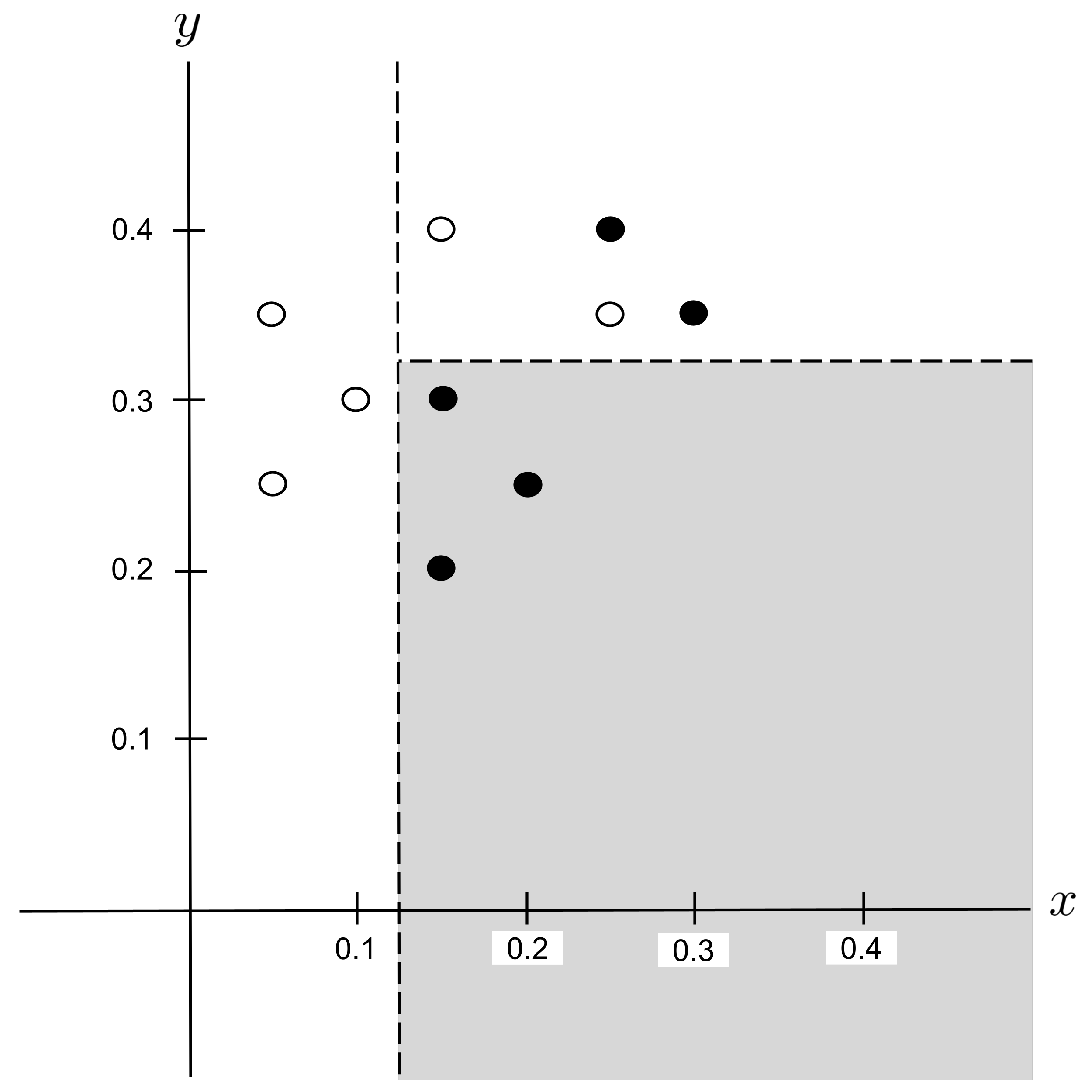
According to the table above, the best split is $x_\textrm{split} = 0.125$ since it decreases the impurity the most. We integrate this split into our decision tree:

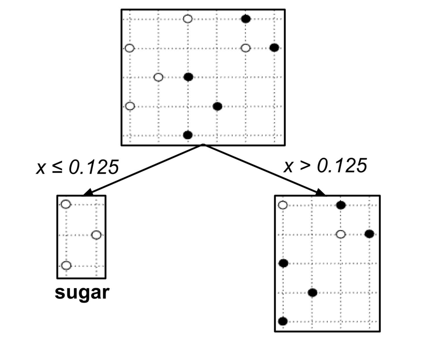
This decision tree can be visualized in the plane as follows:

Worked Example: Split 2

Again, we repeat the process and split any impure leaf nodes in the tree. There is exactly one impure leaf node $(x > 0.125)$ and it contains $5$ shortbread and $2$ sugar cookies, giving an impurity of

To find the possible splits, we first find the distinct values of $x$ and $y$ that are hit by points in this node and put them in order:

The possible splits are the midpoints between consecutive entries in the list above:

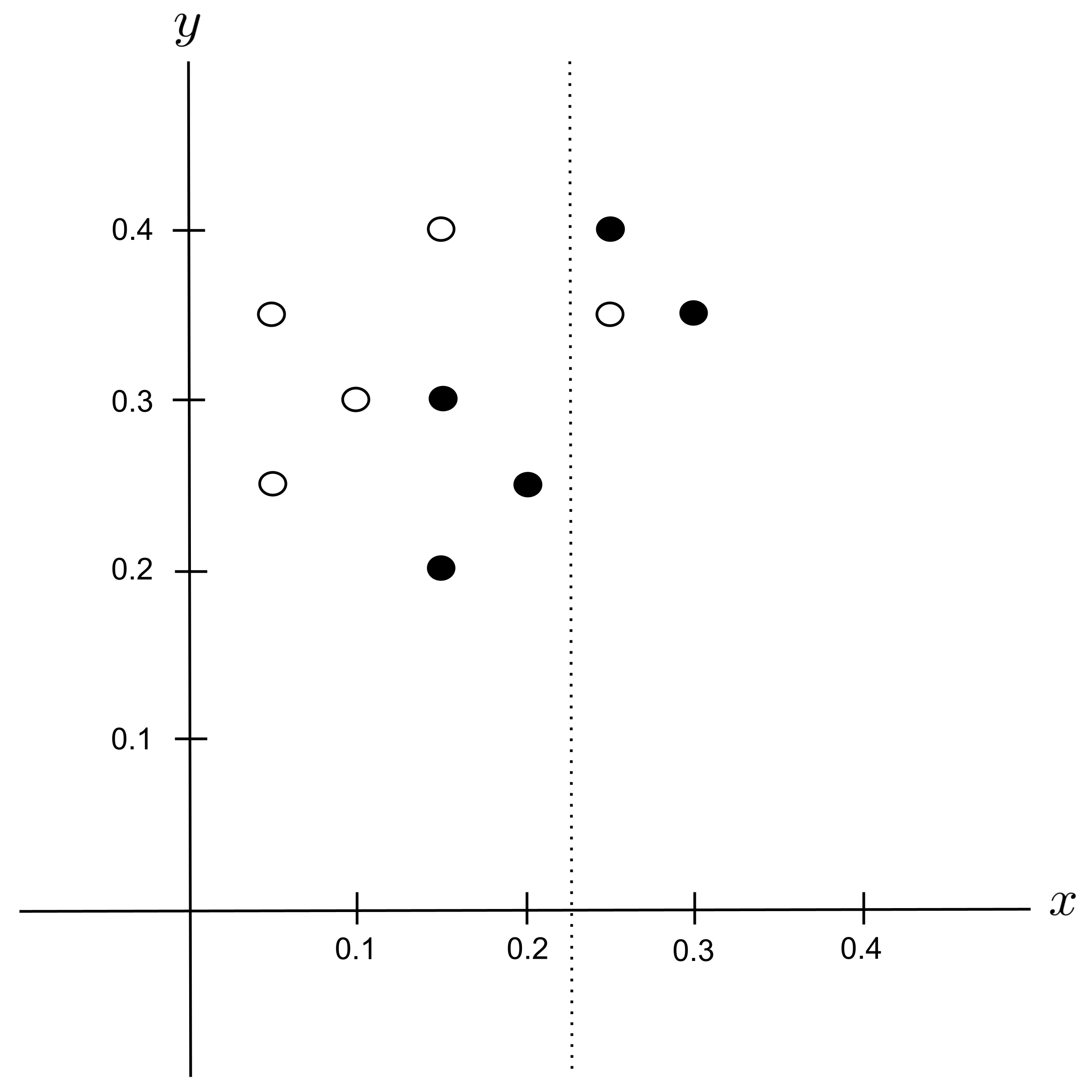
Possible Split: $x_\textrm{split} = 0.175$

Remember that we are only splitting the region covered by the $x > 0.125$ node, which contains $7$ data points. We can ignore the $3$ data points left of the hard dotted line, since they are not contained within the node that we are splitting.

Possible Split: $x_\textrm{split} = 0.225$

Possible Split: $x_\textrm{split} = 0.275$

Possible Split: $y_\textrm{split} = 0.225$

Possible Split: $y_\textrm{split} = 0.275$

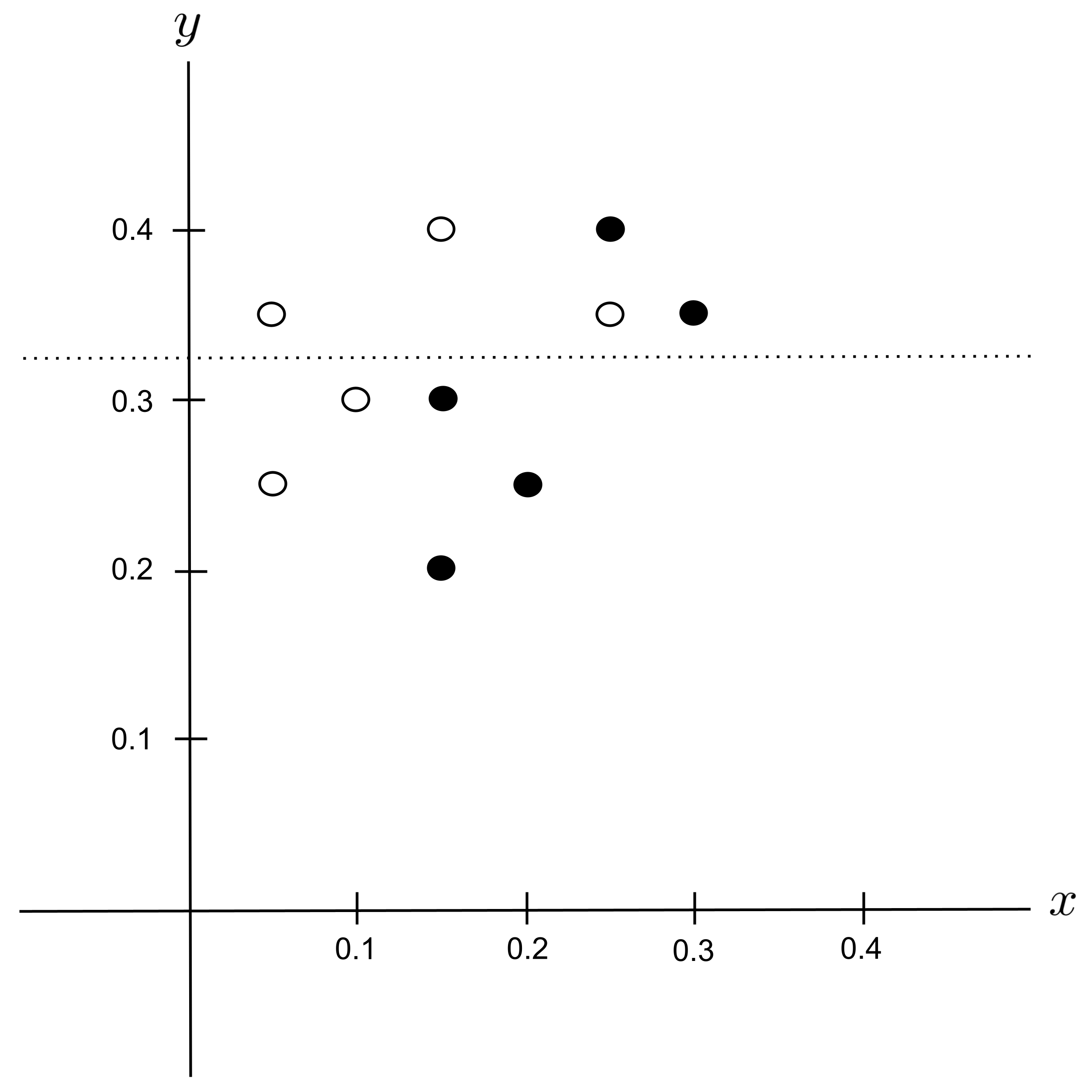
Possible Split: $y_\textrm{split} = 0.325$

Possible Split: $y_\textrm{split} = 0.375$

Best Split

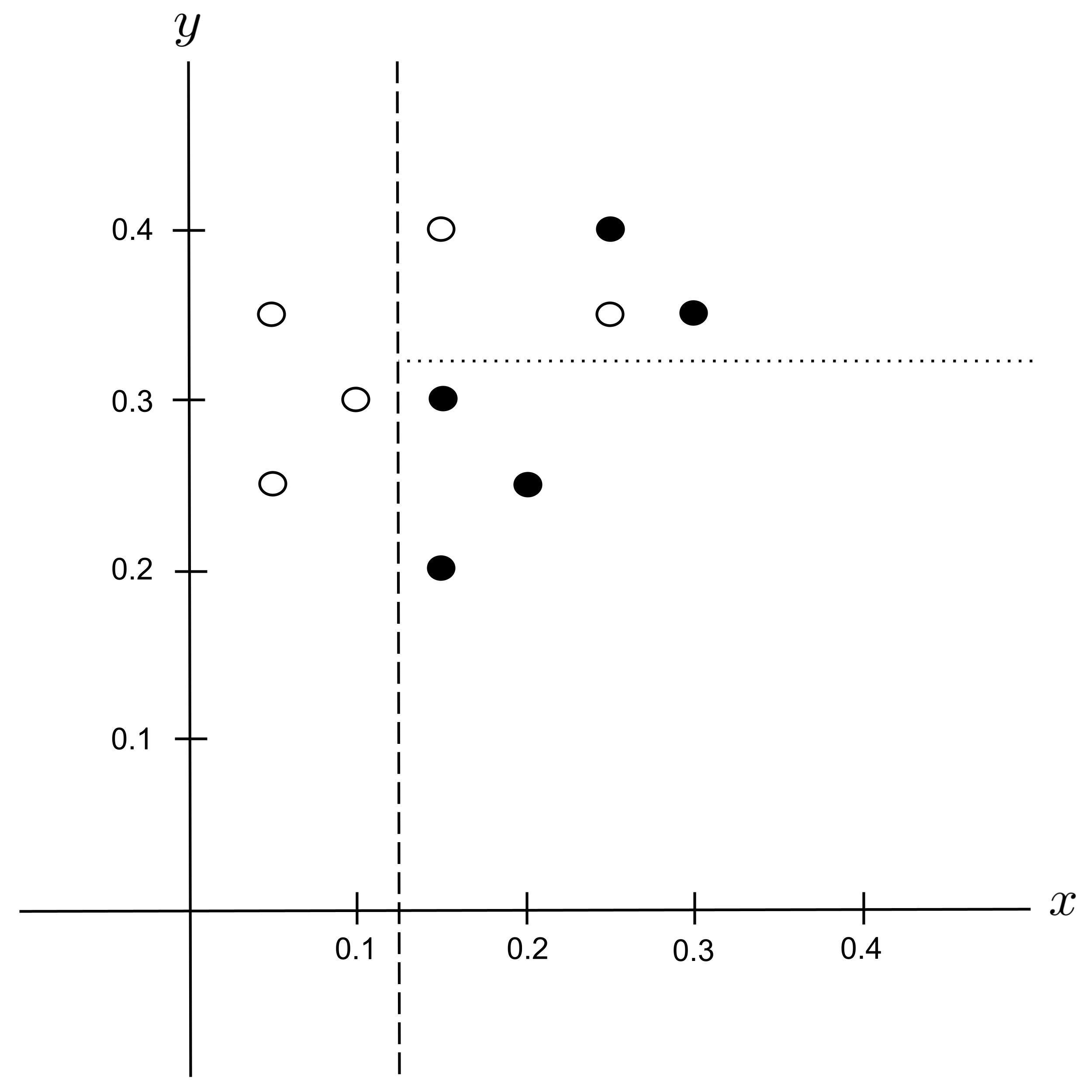
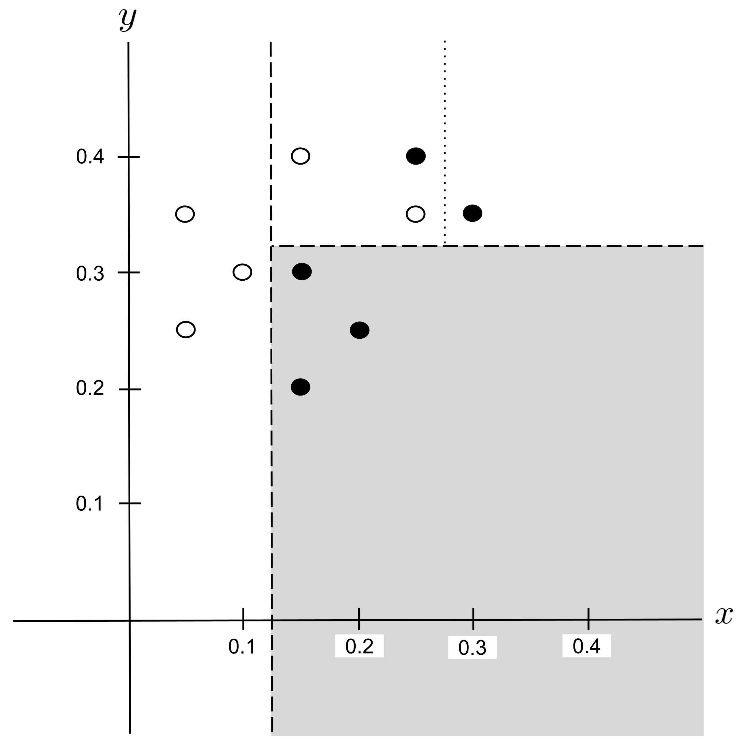
The best split is $y_\textrm{split} = 0.325$ since it decreases the impurity the most.

We integrate this split into our decision tree:

This decision tree can be visualized in the plane as follows:

Worked Example: Split 3

Again, we repeat the process and split any impure leaf nodes in the tree. There is exactly one impure leaf node $(x > 0.125$ $\to$ $y > 0.325)$ and it contains $2$ shortbread and $2$ sugar cookies, giving an impurity of

To find the possible splits, we first find the distinct values of $x$ and $y$ that are hit by points in this node and put them in order:

The possible splits are the midpoints between consecutive entries in the list above:

Possible Split: $x_\textrm{split} = 0.2$

Remember that we are only splitting the region covered by the $x > 0.125$ $\to$ $y > 0.325$ node, which contains $4$ data points. We can ignore the $6$ data points outside of this region, since they are not contained within the node that we are splitting.

Possible Split: $x_\textrm{split} = 0.275$

Possible Split: $y_\textrm{split} = 0.375$

Best Split

This time, there is a tie for the best split: $x_\textrm{split} = 0.2$ and $x_\textrm{split} = 0.275$ both decrease impurity the most.

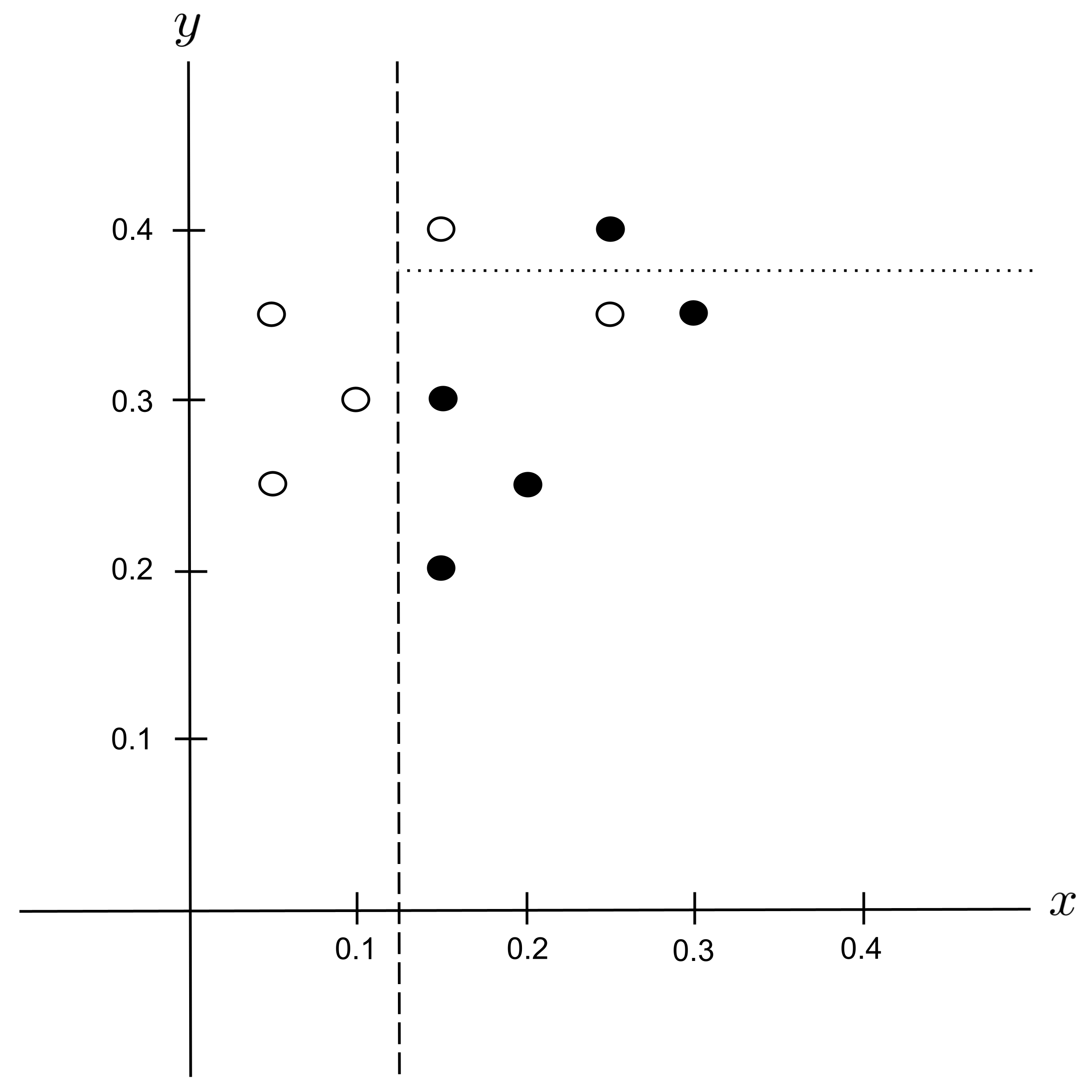
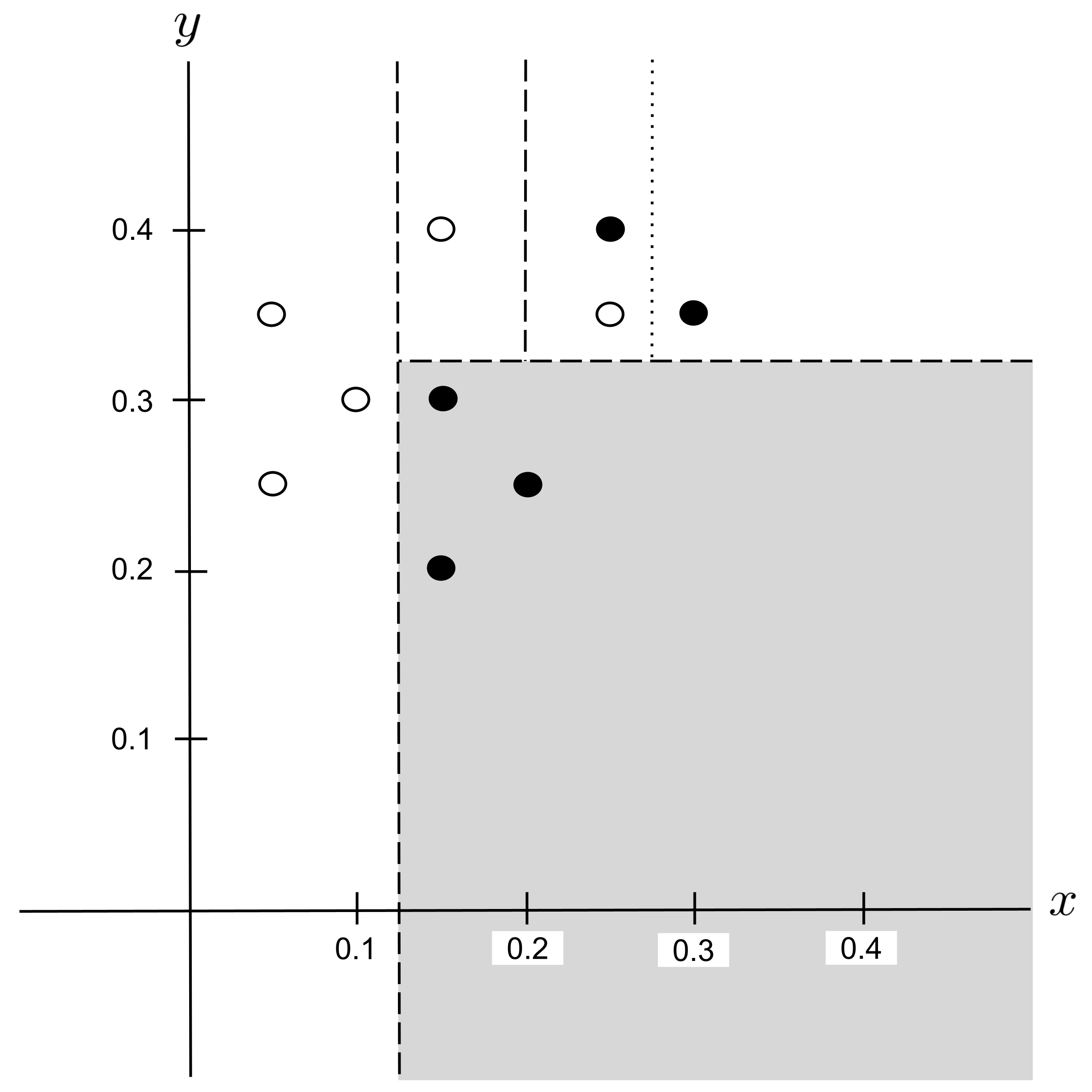
When ties like this occur, it does not matter which split we choose. We will arbitrarily choose the split that we encountered first, $x_\textrm{split} = 0.2,$ and integrate this split into our decision tree:

This decision tree can be visualized in the plane as follows:

Worked Example: Split 4

Again, we repeat the process and split any impure leaf nodes in the tree. There is exactly one impure leaf node $(x > 0.125$ $\to$ $y > 0.325$ $\to$ $x > 0.2)$ and it contains $2$ shortbread and $1$ sugar cookie, giving an impurity of

To find the possible splits, we first find the distinct values of $x$ and $y$ that are hit by points in this node and put them in order:

The possible splits are the midpoints between consecutive entries in the list above:

Possible Split: $x_\textrm{split} = 0.275$

Possible Split: $y_\textrm{split} = 0.375$

Best Split

Again, there is a tie for the best split: $x_\textrm{split} = 0.275$ and $y_\textrm{split} = 0.375$ both decrease impurity the most.

We will arbitrarily choose the split that we encountered first, $x_\textrm{split} = 0.275,$ and integrate this split into our decision tree:

This decision tree can be visualized in the plane as follows:

Worked Example: Split 5

There is only one possibility for the next split, $y_\textrm{split} = 0.375,$ so it may be tempting to select it outright. But remember that we only want splits that lead to a decrease in impurity. So, it’s still necessary to compute the decrease in impurity before selecting this split.

Indeed, the impurity decreases by a positive amount

so we select the split and integrate it into our decision tree:

This decision tree can be visualized in the plane as follows:

No more splits are possible, so we’re done.

Early Stopping

Note that when fitting decision trees, it’s common to stop splitting early so that the tree doesn’t overfit the data. This is often achieved by enforcing

• a maximum depth constraint (i.e. skip over any potential splits that would cause the tree to become deeper than some number of levels), or
• a minimum split size constraint (i.e. do not split any leaf node that contains fewer than some number of data points).

These parameters constrain how far the decision tree can read into the data, similar to how the degree parameter constrains a polynomial regression model and how $k$ constrains a k-nearest neighbors model.

Also note that if we stop splitting early (or if the data set has duplicate points with different classes), we end up with impure leaf nodes. In such cases, impure leaf nodes are considered to predict the majority class of the data points they contain. If there is a tie, then we can go up a level and use the majority class of the parent node.

Random Forests

A common way to improve the performance of decision trees is to select a bunch of random subsets of the data (each containing, say, $\, 50\% \,$ of the data), fit a separate decision tree on each random subset, and then aggregate them together into a hive mind called a random forest. The random forest makes its predictions by

1. allowing each individual decision tree to vote (i.e. make its own prediction), and then
2. choosing whichever prediction received the most votes.

This general approach is called bootstrap aggregating or bagging for short (because a random subset of the data is known as a bootstrap sample). Bootstrap aggregating can be applied to any model, though random forest is the most famous application.

Exercises

1. Implement the example that was worked out above.
2. Construct a leave-one-out cross-validation curve where a maximum depth constraint is varied between $1$ and the number of points in the data set. When the maximum depth is $1,$ the resulting decision tree will contain only one node (a decision "stump" that simply predicts the majority class), and the leave-one-out accuracy will be $0$ (since there will be fewer points in the class of the point that was left out). As usual, the leave-one-out cross-validation curve should reach a maximum somewhere between the endpoints (the endpoints correspond to underfitting or overfitting).
3. Construct a leave-one-out cross-validation curve where a minimum split size constraint is varied between $1$ and one more than the number of points in the data set. It should look like a horizontal reflection of the curve for the maximum depth constraint because increasing the minimum split size has the same pruning effect as decreasing the maximum depth.
4. Construct a leave-one-out cross-validation curve for a random forest, where the number of trees in the forest is varied and each tree is trained on a random sample of $\, 50\% \,$ of the data. You should see the performance increase and asymptote off with the number of trees.
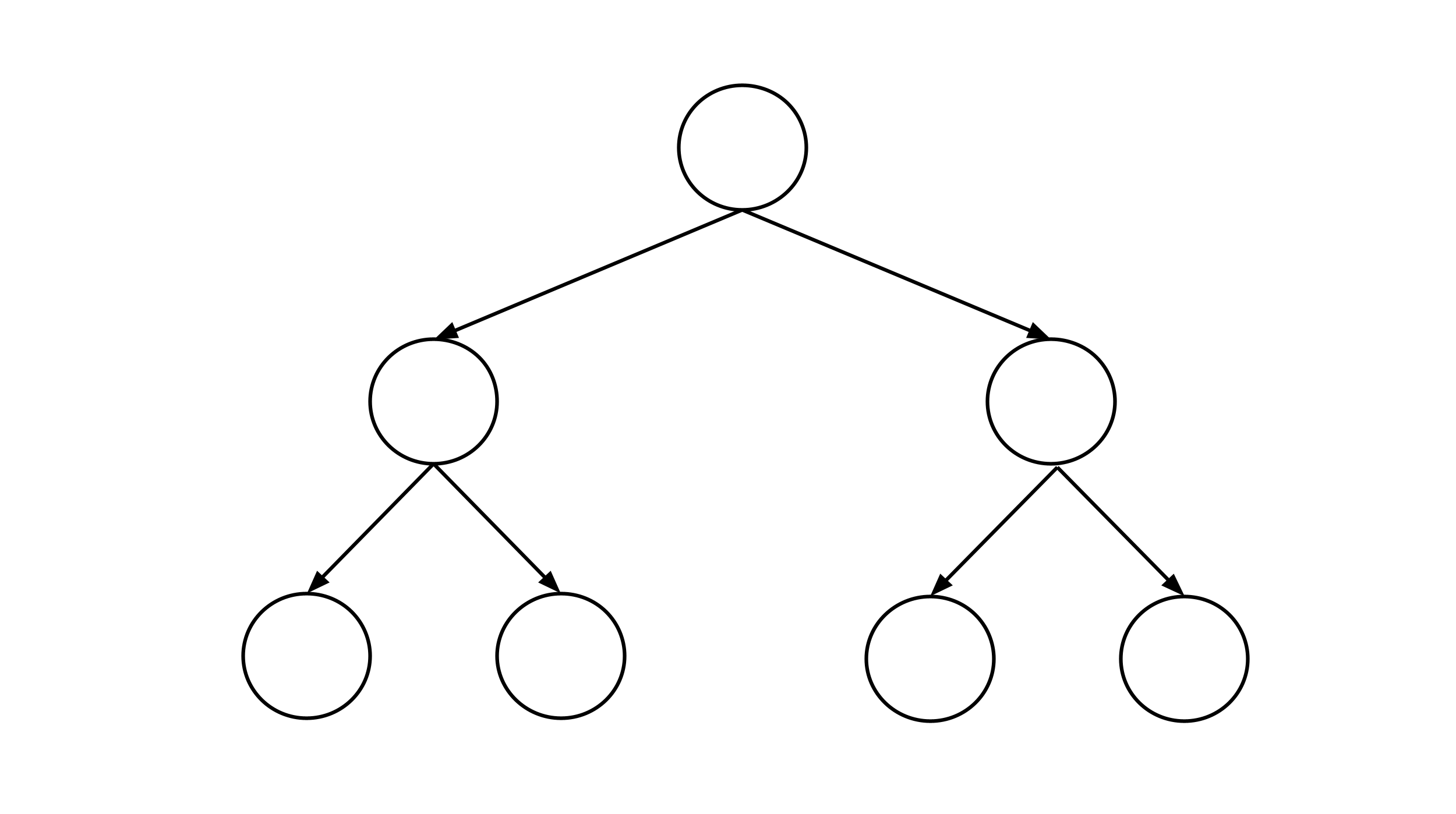
5. Construct a data set that leads to a decision tree that looks like the diagram shown below. Be sure to run your decision tree construction algorithm on the data set to verify the result.
   
   
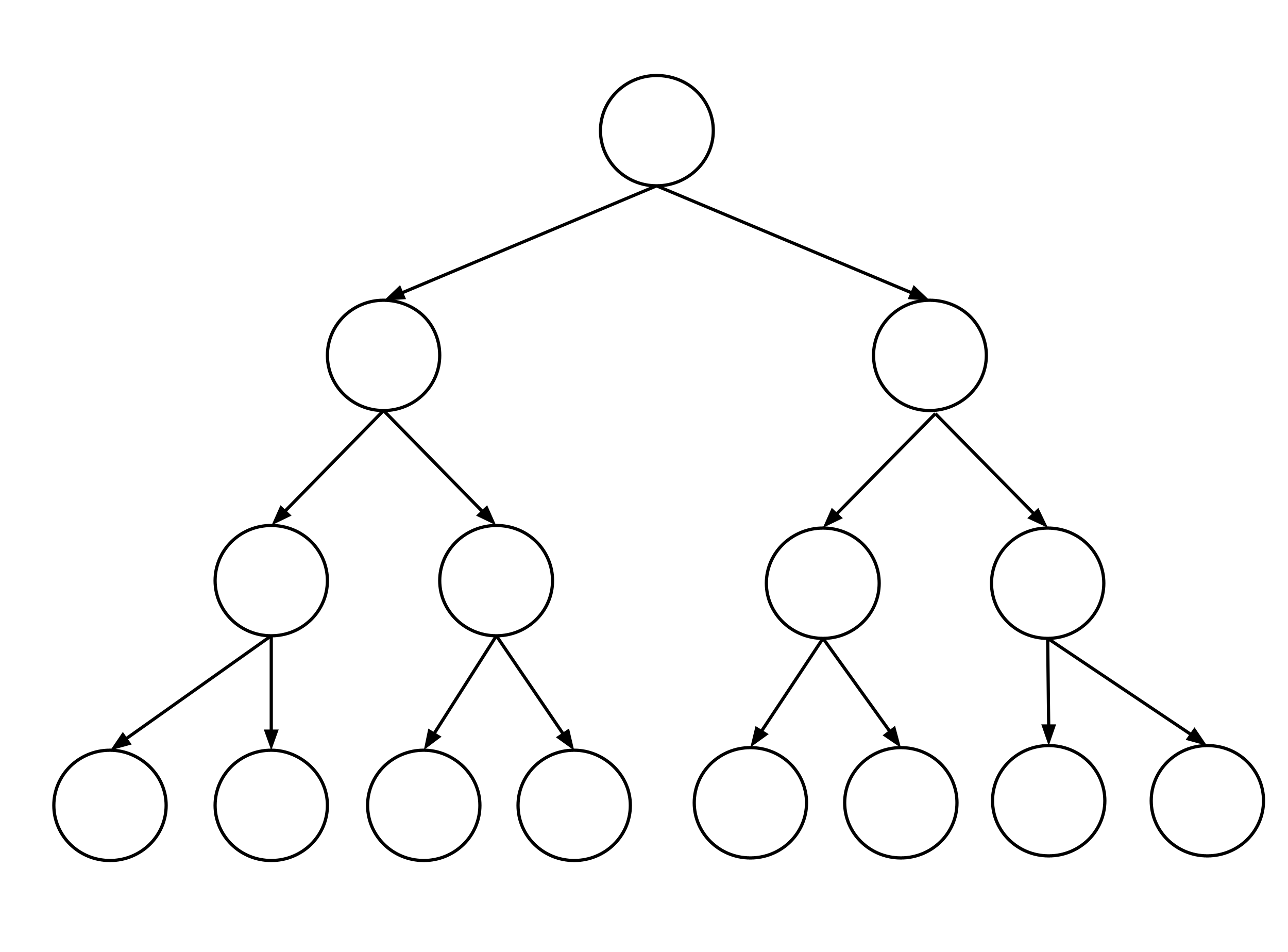
6. Construct a data set that leads to a decision tree that looks like the diagram shown below. Be sure to run your decision tree construction algorithm on the data set to verify the result.
   
   

This post is a chapter in the book Introduction to Algorithms and Machine Learning: from Sorting to Strategic Agents. Suggested citation: Skycak, J. (2022). Decision Trees. Introduction to Algorithms and Machine Learning: from Sorting to Strategic Agents. https://justinmath.com/decision-trees/