Dijkstra’s Algorithm for Distance and Shortest Paths in Weighted Graphs

by Justin Skycak on February 03, 2022

Computing spatial relationships between nodes when edges no longer represent unit distances.

This post is a chapter in the book Introduction to Algorithms and Machine Learning: from Sorting to Strategic Agents. Suggested citation: Skycak, J. (2022). Dijkstra's Algorithm for Distance and Shortest Paths in Weighted Graphs. Introduction to Algorithms and Machine Learning: from Sorting to Strategic Agents. https://justinmath.com/dijkstras-algorithm-for-distance-and-shortest-paths-in-weighted-graphs/

In a weighted graph, every edge is assigned a value called a weight.

Initializing a Weighted Graph

For example, consider the following weighted graph:

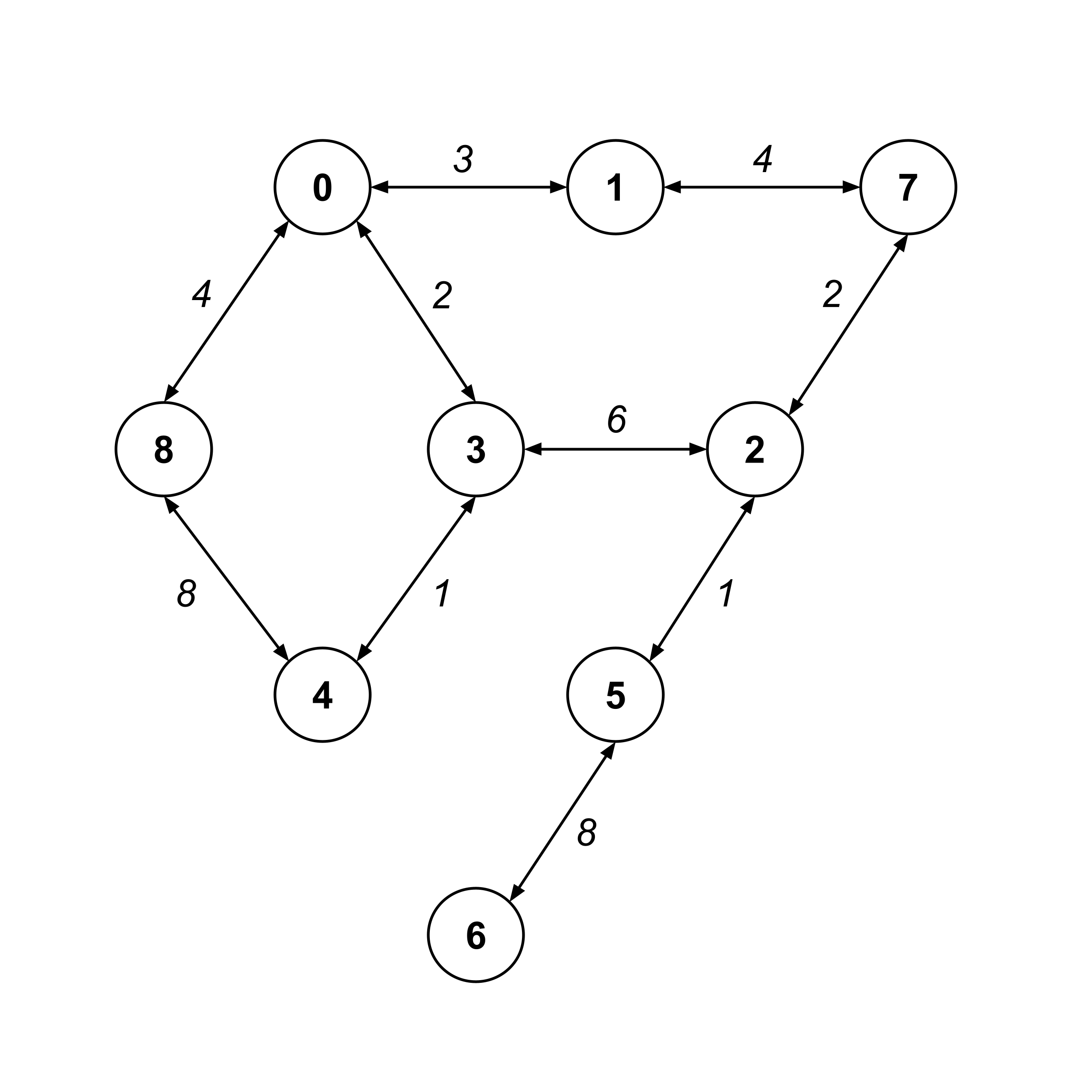
A weighted graph can be initialized with a weights dictionary instead of an edges list. The edges list just had a list of edges, whereas the weights dictionary will have its keys as edges and its values as the weights of those edges.


>>> weights = {
    (0,1): 3, (1,0): 3,
    (1,7): 4, (7,1): 4,
    (7,2): 2, (2,7): 2,
    (2,5): 1, (5,2): 1,
    (5,6): 8, (6,5): 8,
    (0,3): 2, (3,0): 2,
    (3,2): 6, (2,3): 6,
    (3,4): 1, (4,3): 1,
    (4,8): 8, (8,4): 8,
    (8,0): 4, (0,8): 4
}

>>> weighted_graph = WeightedGraph(weights)

Distance and Shortest Paths in Weighted Graphs

In a weighted graph, the distance between two nodes is the sum of the weights on the shortest path between them. For example, the distance from node $8$ to node $4$ is $7$ because the shortest path is $8 \stackrel{4}{\to} 0 \stackrel{2}{\to} 3 \stackrel{1}{\to} 4.$

In particular, notice that the shortest path is NOT $8 \stackrel{8}{\to} 4$ because the distance along this path is $8.$


>>> [weighted_graph.calc_distance(8,n) for n in range(9)]
[4, 7, 12, 6, 7, 13, 21, 11, 0]

>>> weighted_graph.calc_shortest_path(8,4)
[8, 0, 3, 4]

>>> weighted_graph.calc_shortest_path(8,7)
[8, 0, 1, 7]

>>> weighted_graph.calc_shortest_path(8,6)
[8, 0, 3, 2, 5, 6]

Dijkstra's Algorithm for Distance

The underlying algorithms for calc_distance and calc_shortest_path are a bit more complicated for weighted graphs than for unweighted graphs.

To implement calc_distance(from_idx, to_idx) we need to use Dijkstra’s algorithm, which works by assigning each node an initial guess for its distance and then repeatedly updating those guesses until they actually represent the distances to those nodes.

When setting initial guesses, the "from" node is assigned a distance value of $0$, and all other nodes are assigned distance values of $\infty$ (just use a large number like $9999999999$).
Set the current_node to be the "from" node.
Loop through the current_node's unvisited children and update their distances as child.distance = min(child.distance, current_node.distance + edge_weight).
Update the current_node to be the unvisited node with the smallest distance value (not necessarily a child node).
If the ending node has not been visited yet, then return to step $3.$
Return the distance attribute of the "to" node.

Let’s demonstrate each iteration of Dijkstra’s algorithm when computing the distance from node $8$ to node $6.$

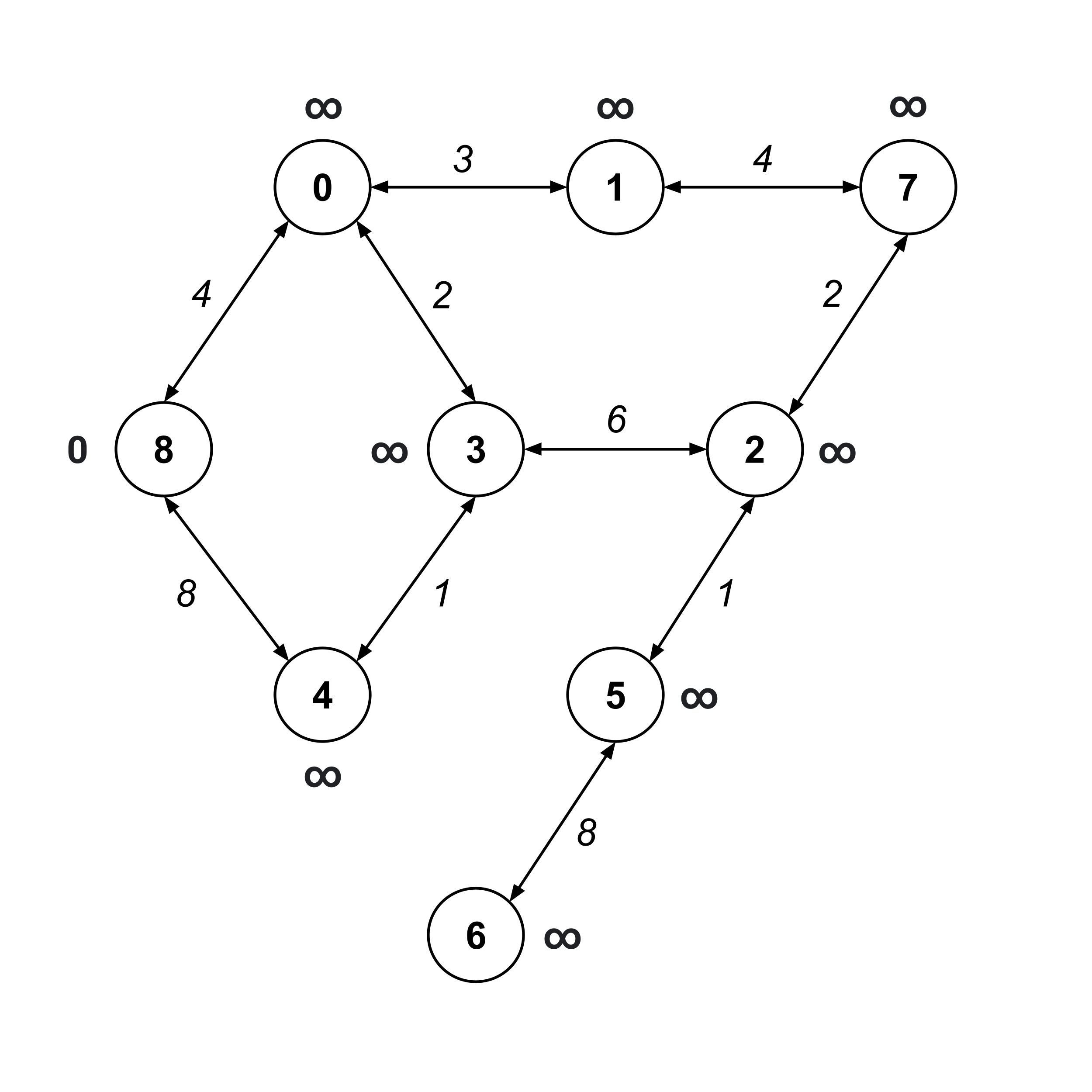
First, we set the initial guesses for the distance values. Since we’re starting at node $8,$ we already know that it’s a distance of $0$ from itself. All the other nodes get initial guesses of infinity.

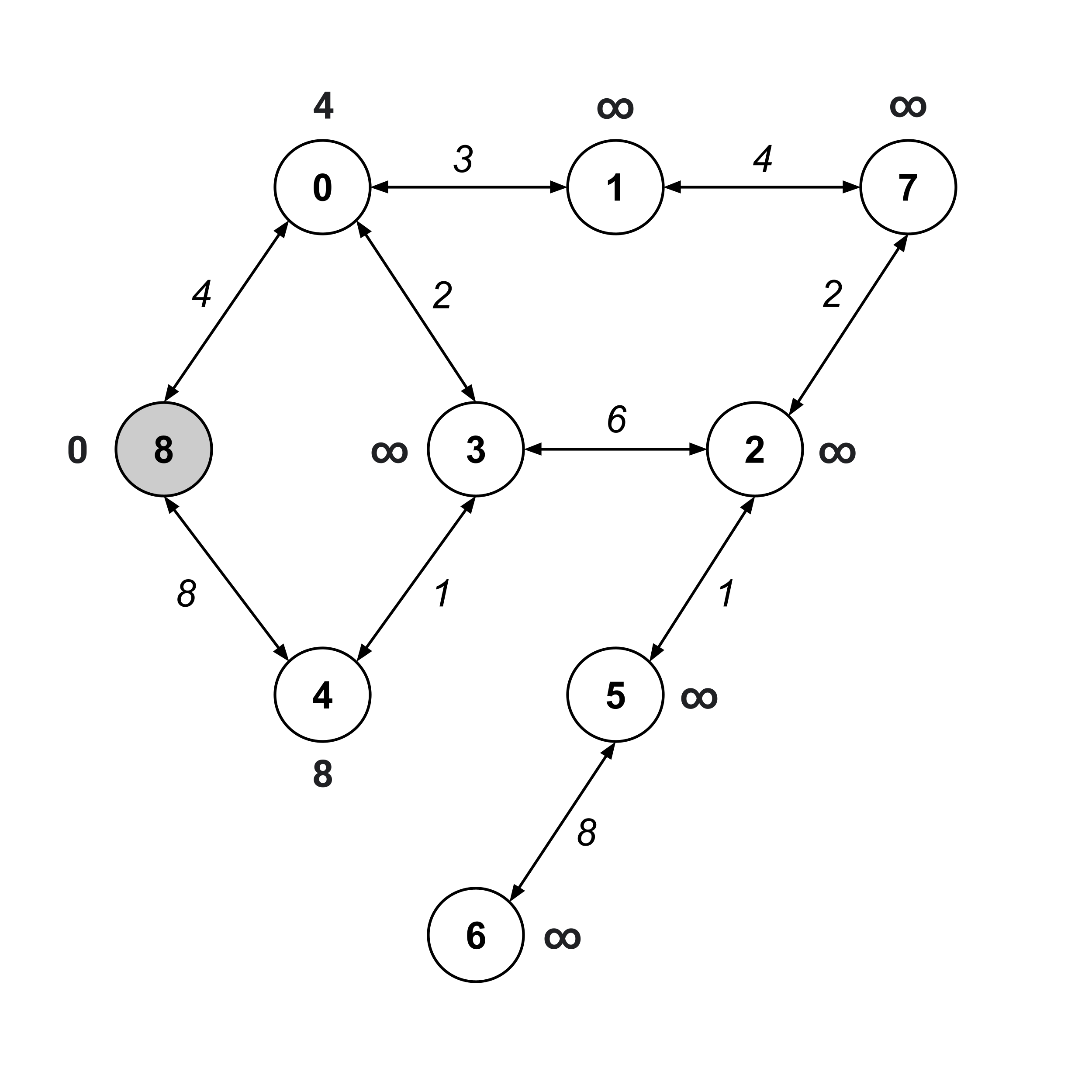
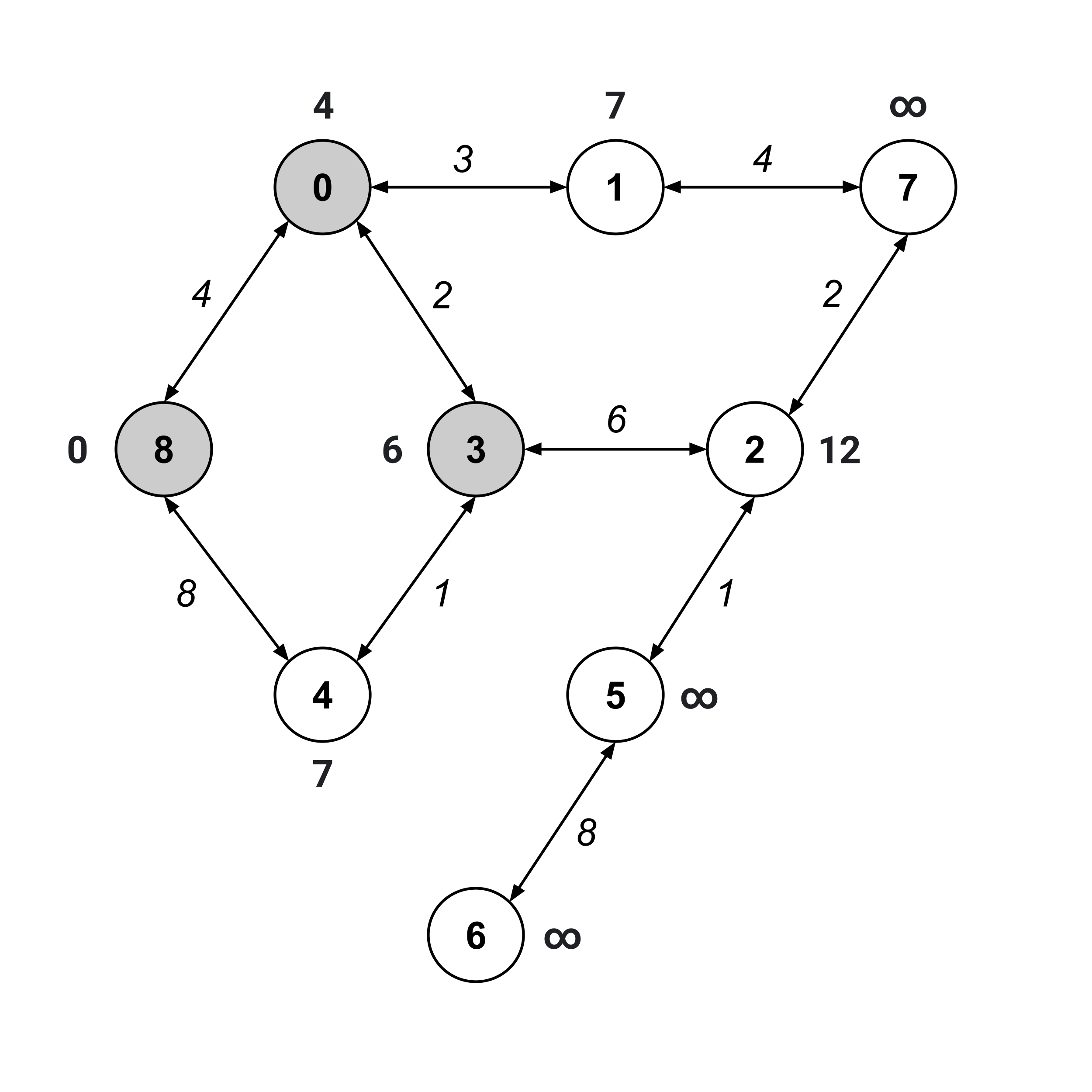
Now, we visit node 8 (the “from” node) and update the distance values on its children.

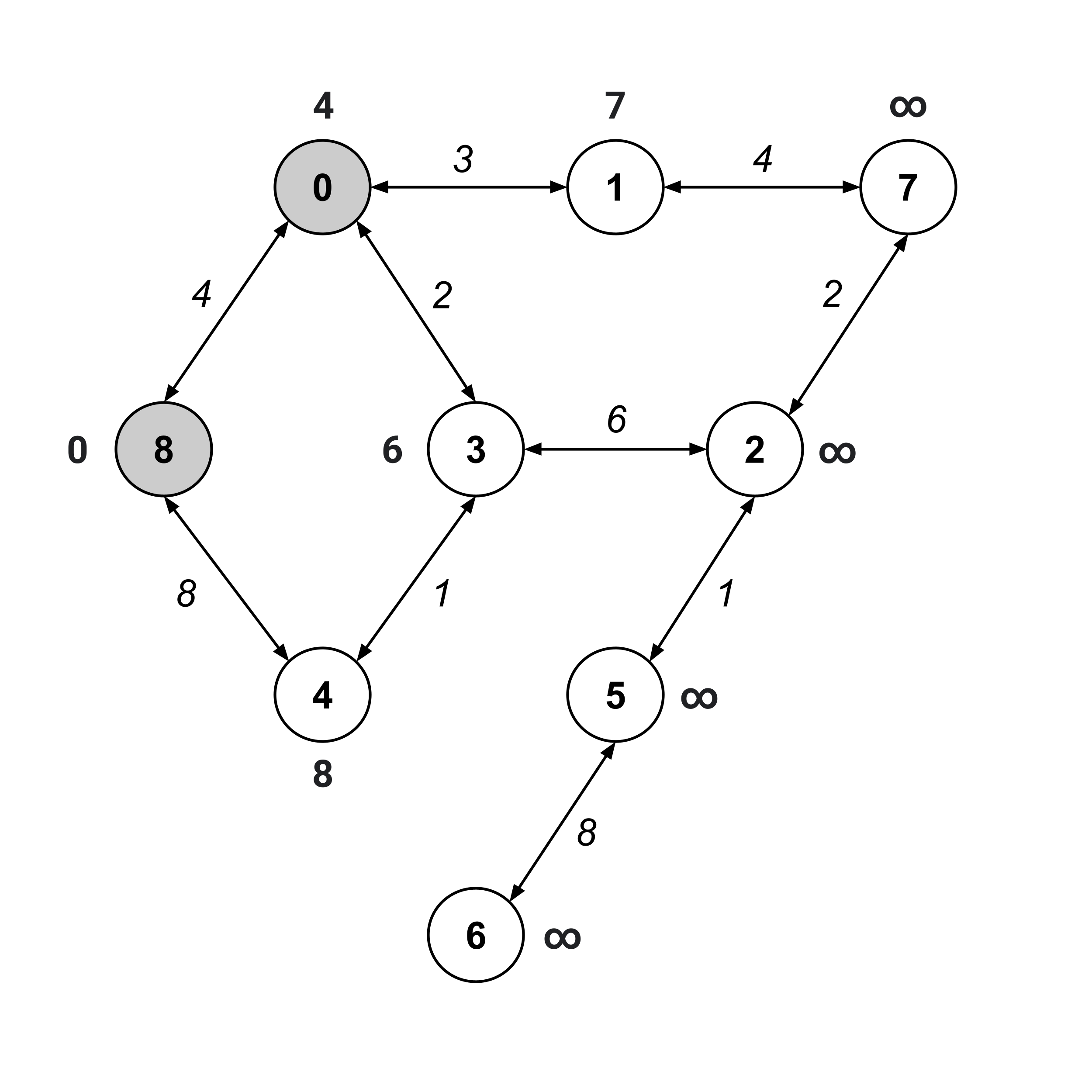
The next node we visit should be the unvisited node with the smallest distance value. This would be node $0,$ whose distance value is $4.$ We visit this node and update the distance values on its unvisited children.

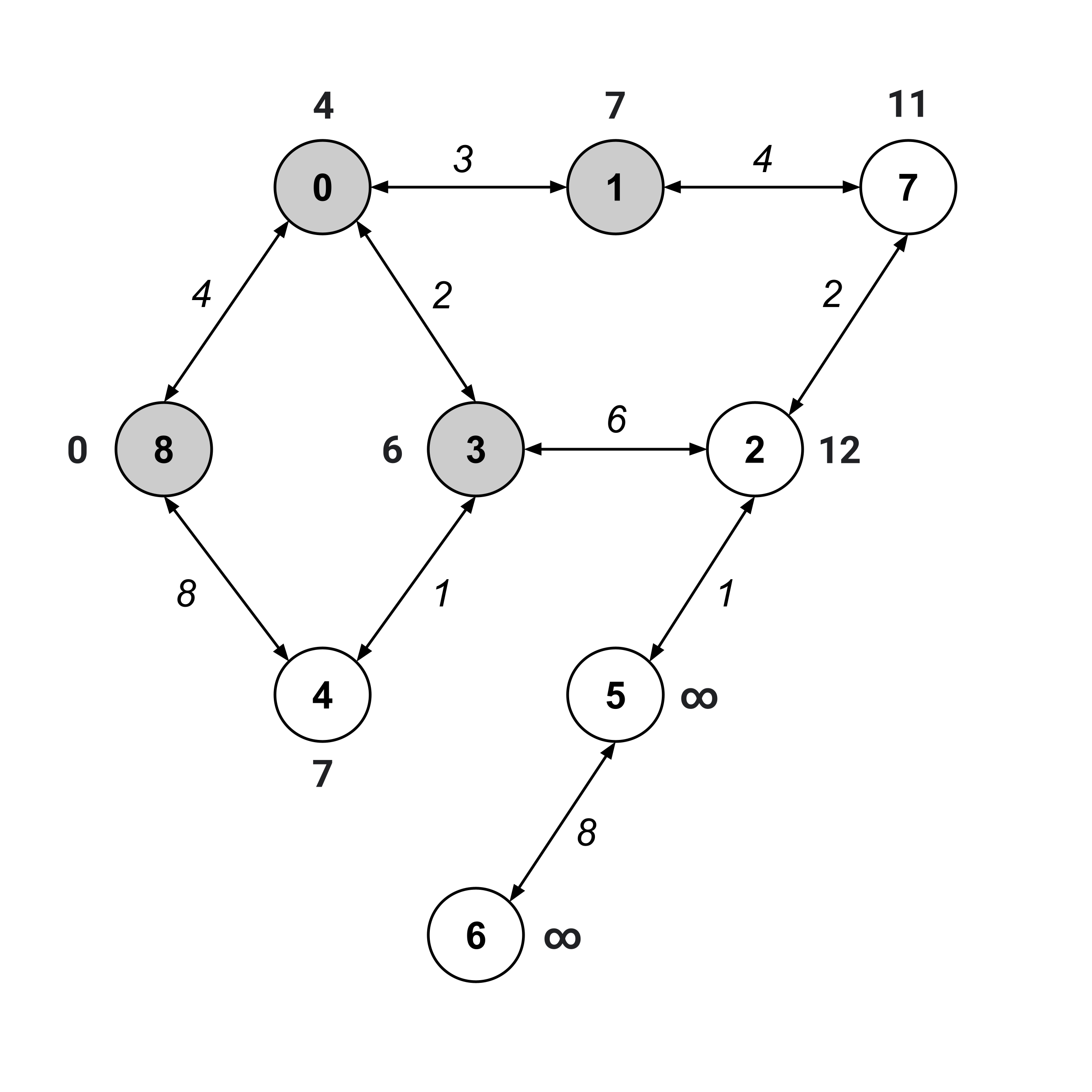
Again, we visit the unvisited node with the smallest distance value. This time, it’s node $3.$

Notice that when we update the distance values on its unvisited children, node $4$’s distance value decreases from $8$ to $7.$ Whenever a distance value decreases like this, it means that the nodes we’ve traversed contain a shorter path than a path we found earlier.

In our first iteration, we found a path $8 \stackrel{8}{\to} 4$ with distance $8.$ Now, we found a path $8 \stackrel{4}{\to} 0 \stackrel{2}{\to} 3 \stackrel{1}{\to} 4$ with distance $7.$

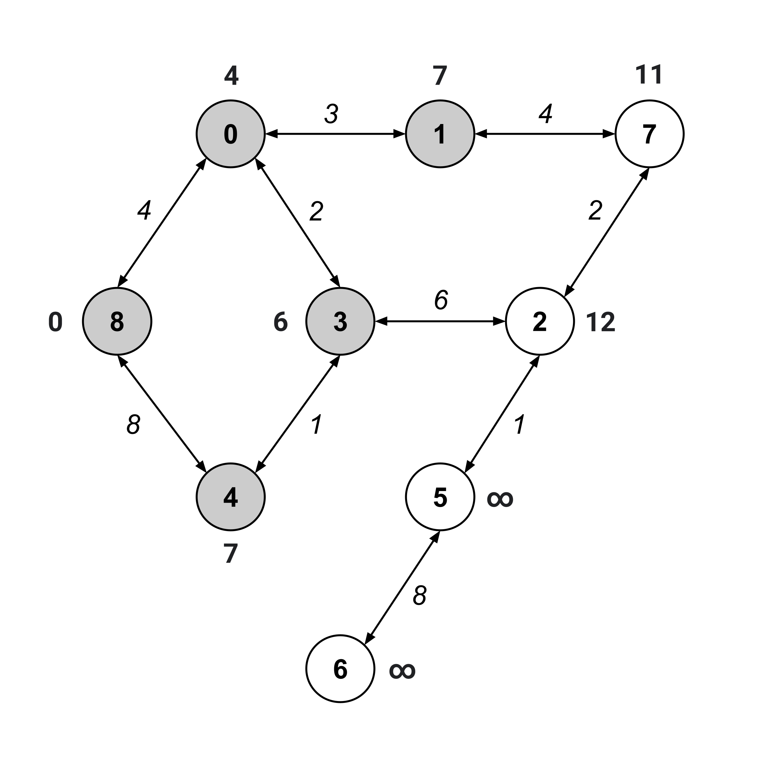
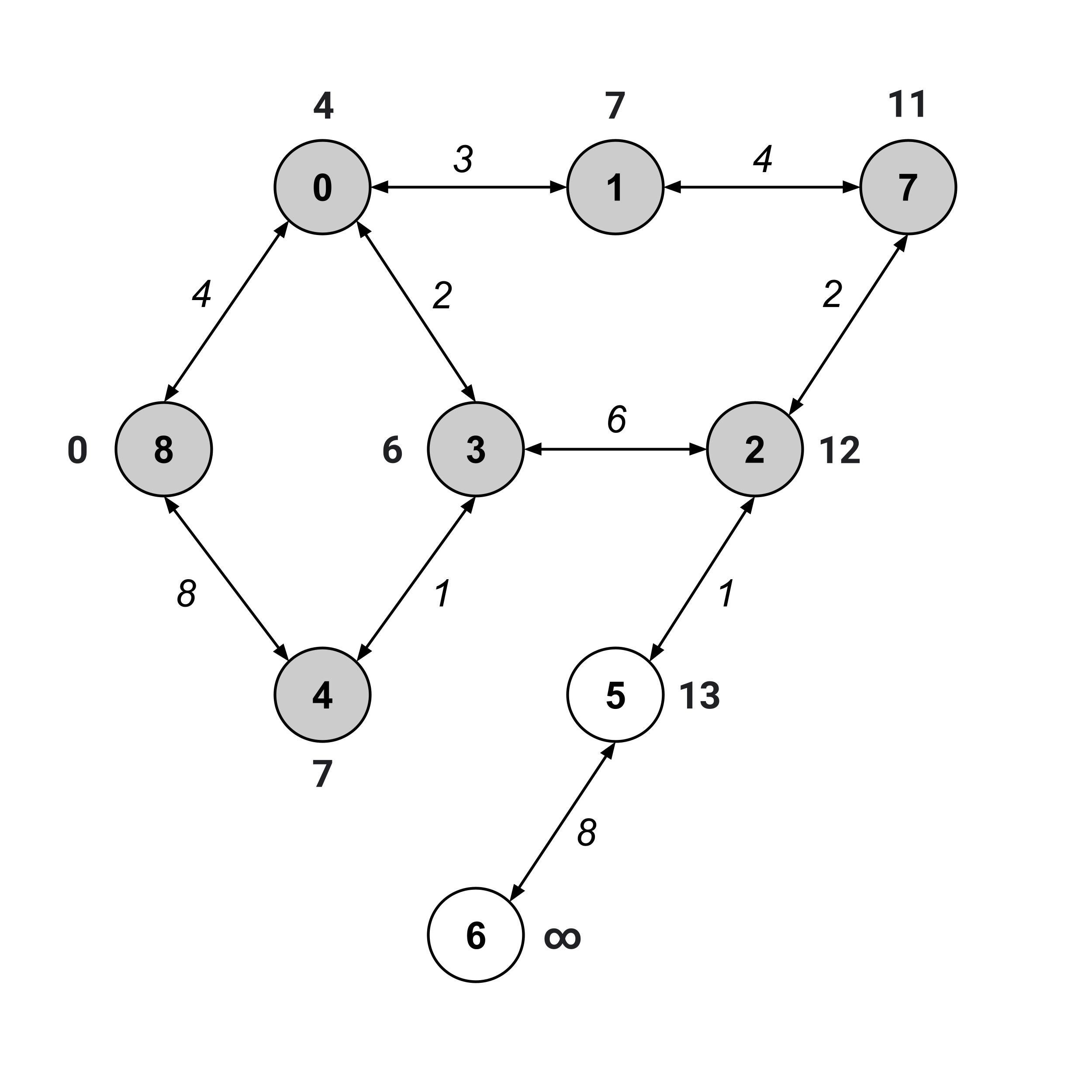
As usual, we visit the unvisited node with the smallest distance value. This time, we can visit either node $1$ or node $4$ (they are the unvisited nodes with the smallest distance values). We’ll arbitrarily choose to visit node $1$ and update the distance values of its children.

We keep on repeating this same procedure until the “to” node (node $6$) has been visited.

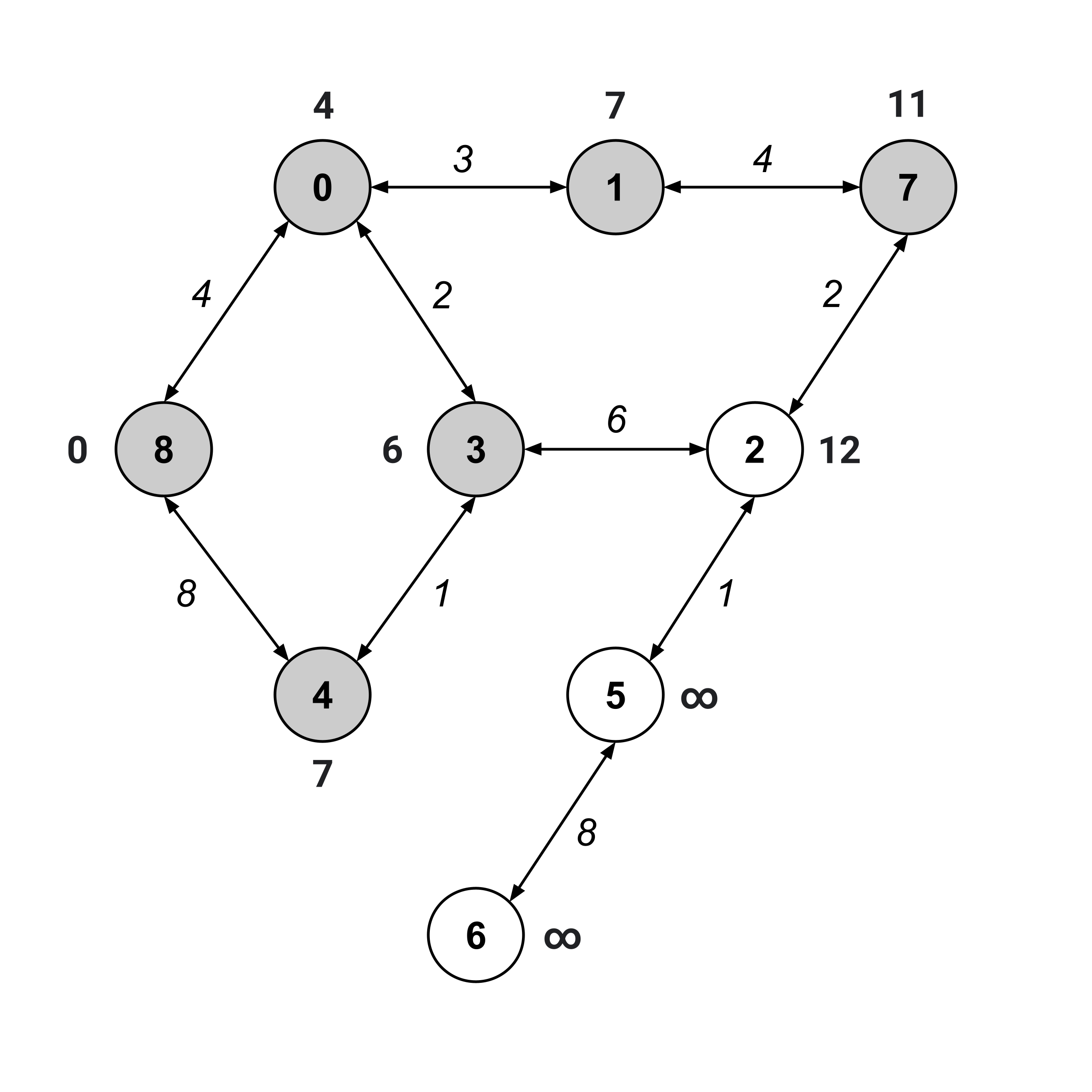
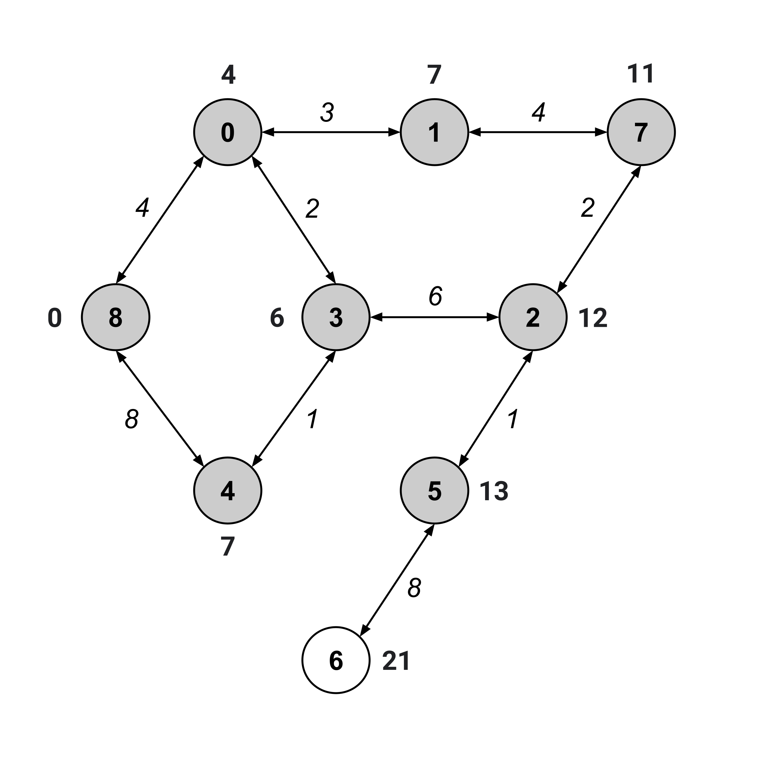
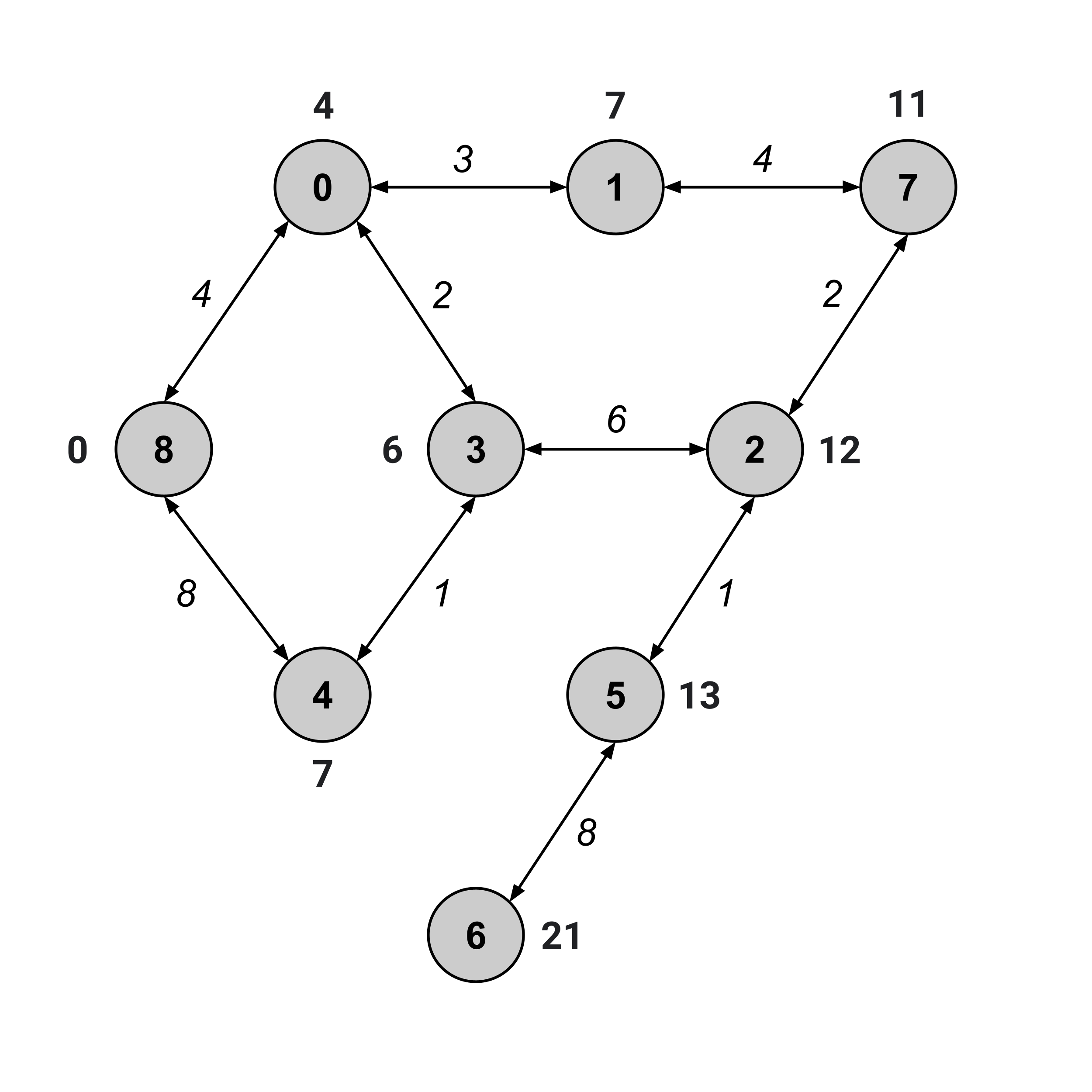
We’ve visited node $6,$ and its distance value is $21.$ This means that the distance from node 8 to node 6 is $21.$

Computing Shortest Paths via the Shortest-Path Tree

But what is the specific shortest path from node $8$ to node $6$ that gives us this distance of $21?$

To find the shortest path, we first construct the shortest-path tree by discarding any edge (a,b) whose weight does not match the corresponding difference between distance values, b.distance - a.distance.

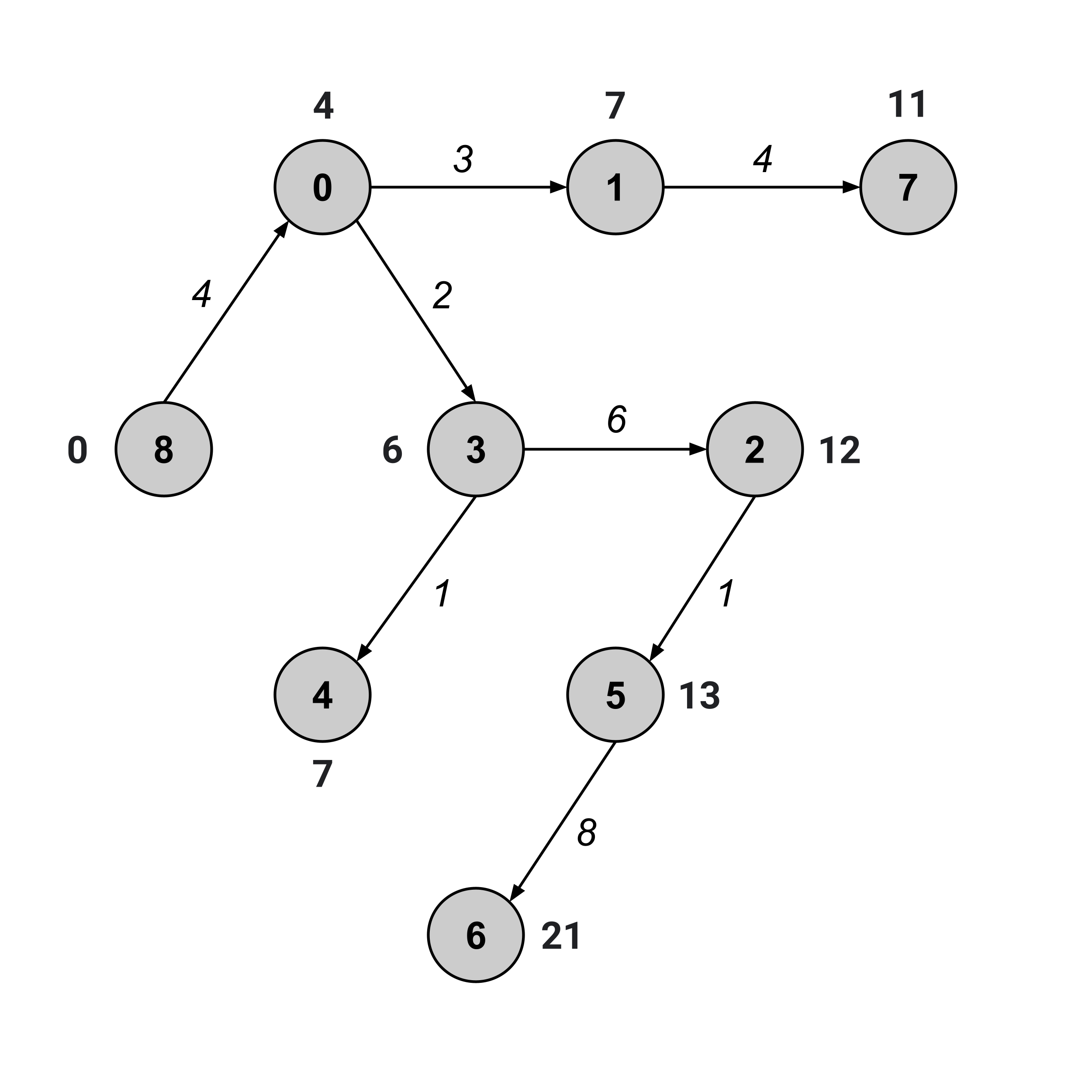
Once we have the shortest-path tree, we’ve effectively reduced our problem down to a problem that we’ve already solved: finding the shortest path between two nodes in an unweighted graph.

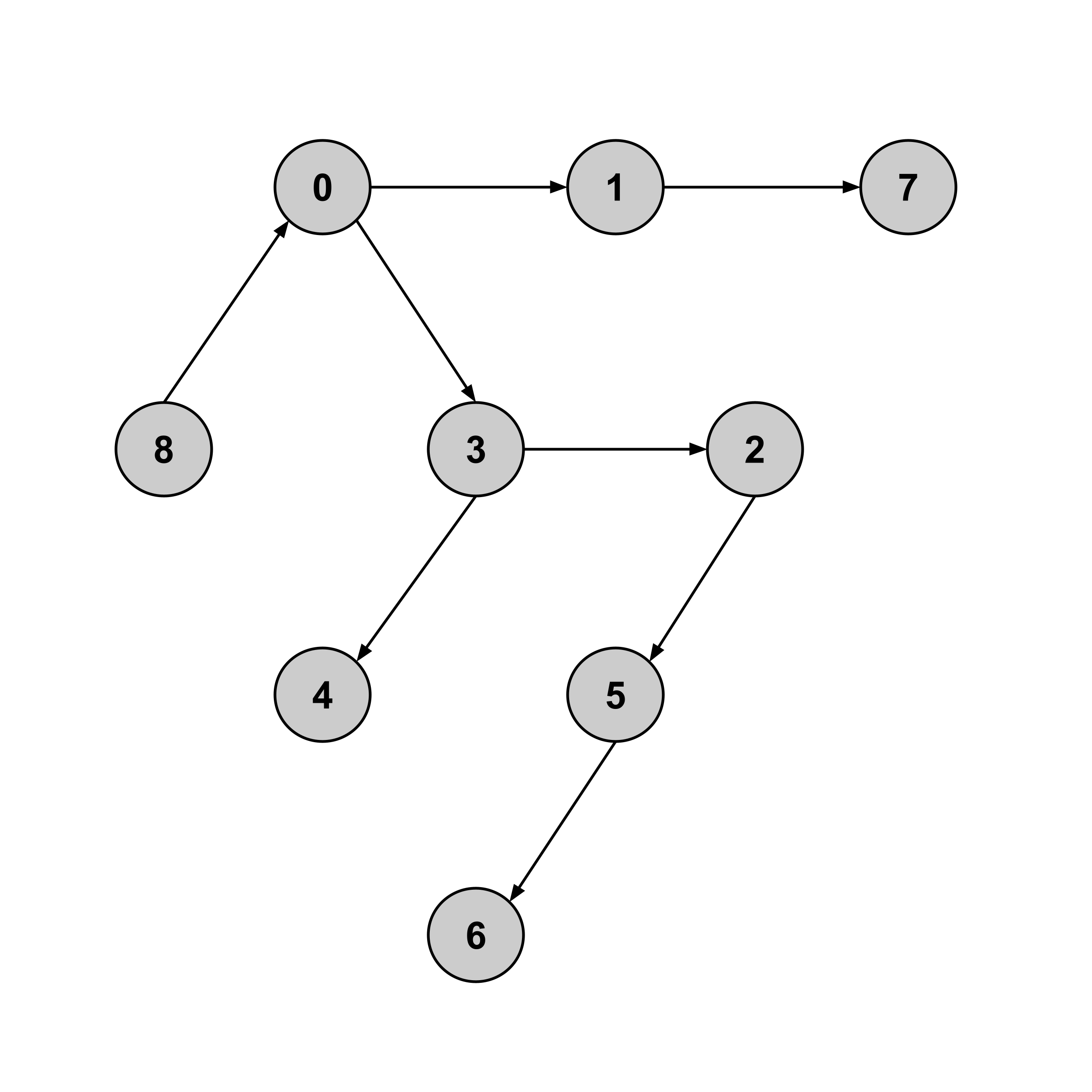
Indeed, we can see that the shortest path from node $8$ to node $6$ in the tree above is given by $8 \to 0 \to 3 \to 2 \to 5 \to 6.$ And indeed, in the weighted graph, the sum of weights along this path is $21.$

Exercises

Implement a WeightedGraph class with the methods calc_distance and calc_shortest_path. As always, be sure to write tests.