Backpropagation

by Justin Skycak on February 06, 2022

A convenient technique for computing gradients in neural networks.

This post is a chapter in the book Introduction to Algorithms and Machine Learning: from Sorting to Strategic Agents. Suggested citation: Skycak, J. (2022). Backpropagation. Introduction to Algorithms and Machine Learning: from Sorting to Strategic Agents. https://justinmath.com/backpropagation/

The most common method used to fit neural networks to data is gradient descent, just like we did have done previously for simpler models. The computations are significantly more involved for neural networks, but an algorithm called backpropagation provides a convenient framework for computing gradients.

Core Idea

The backpropagation algorithm leverages two key facts:

If you know $\dfrac{\partial \textrm{RSS}}{\partial \sigma(\Sigma)}$ for the output $\sigma(\Sigma)$ of a neuron, then you can easily compute $\dfrac{\partial \textrm{RSS}}{\partial w}$ for any weight $w$ that the neuron receives from a neuron in the previous layer.
If you know $\dfrac{\partial \textrm{RSS}}{\partial \sigma(\Sigma)}$ for all neurons in a layer, then you can piggy-back off the result to compute $\dfrac{\partial \textrm{RSS}}{\partial \sigma(\Sigma)}$ for all neurons in the previous layer.

With these two facts in mind, the backpropagation algorithm consists of the following three steps:

Forward propagate neuron activities. Compute $\Sigma$ and $\sigma(\Sigma)$ for all neurons in the network, starting at the input layer and repeatedly piggy-backing off the results to compute $\Sigma$ and $\sigma(\Sigma)$ for all neurons in the next layer.
Backpropagate neuron output gradients. Compute $\dfrac{\partial \textrm{RSS}}{\partial \sigma(\Sigma)}$ for all neurons, starting with the output layer and then repeatedly piggy-backing off the results to compute $\dfrac{\partial \textrm{RSS}}{\partial \sigma(\Sigma)}$ in the previous layer.
Expand neuron output gradients to weight gradients. Compute $\dfrac{\partial \textrm{RSS}}{\partial w}$ for all weights in the neural network by piggy-backing off of $\dfrac{\partial \textrm{RSS}}{\partial \sigma(\Sigma)}$ for the neuron that receives the weight.

Forward Propagation of Neuron Activities

Let’s formalize these steps mathematically. First, we denote the following quantities:

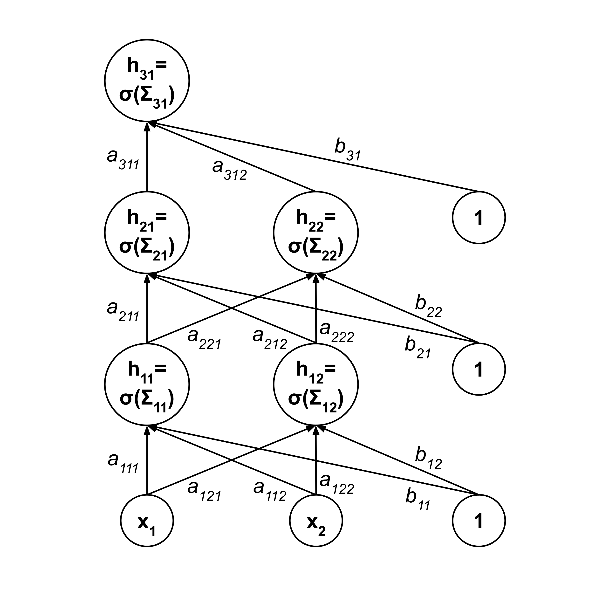
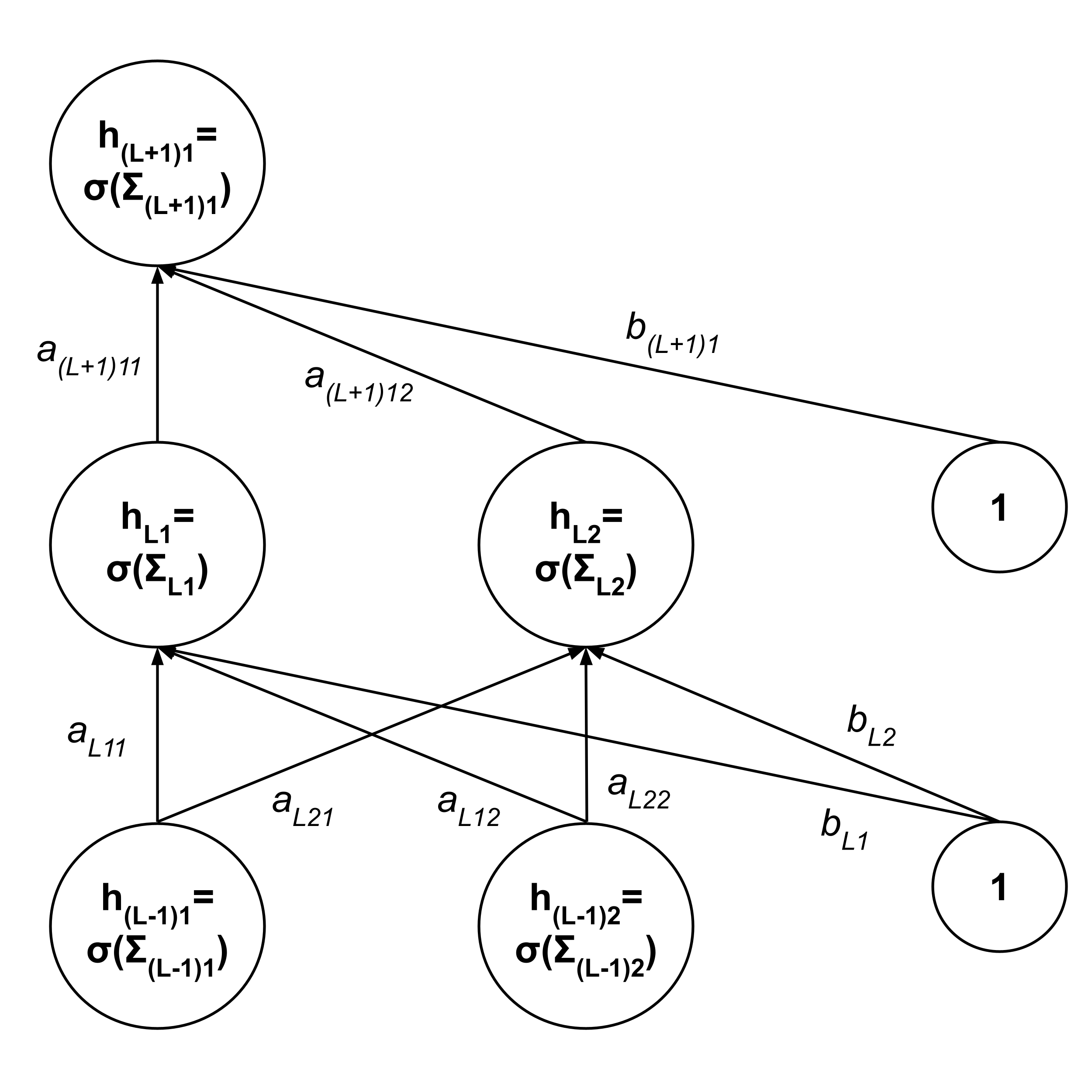
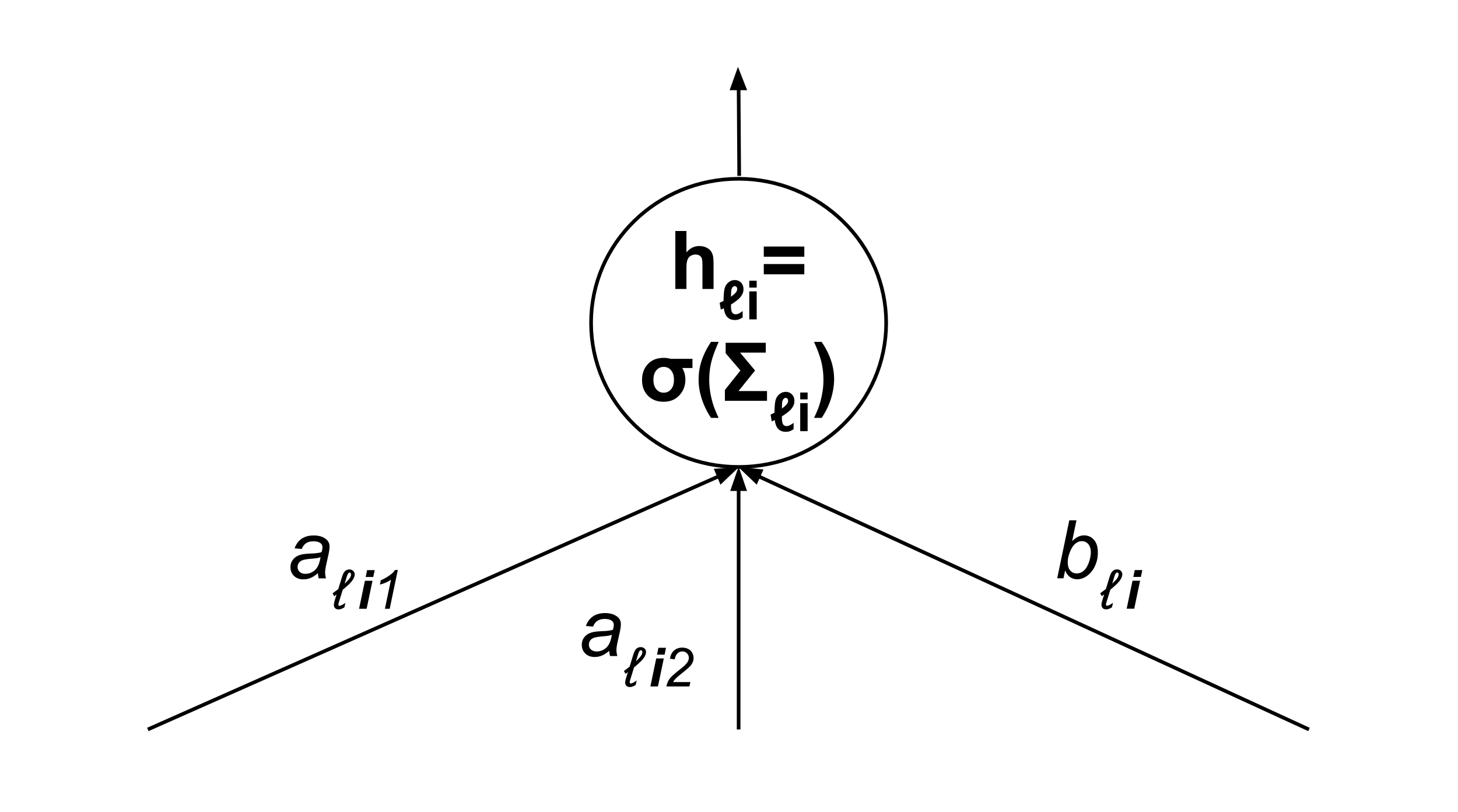
$\vec x = \begin{bmatrix} x_{1} \\ x_{2} \\ \vdots \end{bmatrix}$ are the inputs to the neural network, and $f(\vec x)$ is the output of the neural network.
$\vec \Sigma_\ell = \begin{bmatrix} \Sigma_{\ell 1} \\ \Sigma_{\ell 2} \\ \vdots \end{bmatrix}$ are the inputs to the neurons in the $\ell$th layer, and $\vec h_\ell = \begin{bmatrix} h_{\ell 1} \\ h_{\ell 2} \\ \vdots \end{bmatrix}$ are the outputs of the neurons in the $\ell$th layer. If the activation function of these neurons is $\sigma,$ then $\vec h_\ell = \sigma \left( \vec \Sigma_\ell \right).$
The input layer is the $0$th layer, there are $L$ hidden layers between the input and output layers, and the output layer is the $(L+1)$th layer. Note that this means $\vec h_0 = \vec x$ and $h_{L+1} = f(\vec x).$
$A_\ell = \begin{bmatrix} a_{\ell 11} & a_{\ell 12} & \cdots \\ a_{\ell 21} & a_{\ell 22} & \cdots \\ \vdots && \vdots && \ddots \end{bmatrix}$ is the matrix of connection weights between the non-bias neurons in the $\ell$th layer and the next layer, and $\vec b_\ell = \begin{bmatrix} b_{\ell 1} \\ b_{\ell 2} \\ \vdots \end{bmatrix}$ are the connection weights between the bias neuron in the $\ell$th layer and the neurons in the next layer.

The following diagram may aid in remembering what each symbol represents.

Using the terminology introduced above, we can state the forward propagation step as follows:

$\begin{align*} \vec \Sigma_1 &= A_1 \vec x + \vec b_1 \\[3pt] \vec h_1 &= \sigma \left( \vec \Sigma_1 \right) \\[10pt] \vec \Sigma_2 &= A_2 \vec h_1 + \vec b_2 \\[3pt] \vec h_2 &= \sigma \left( \vec \Sigma_2 \right) \\[10pt] \vec \Sigma_3 &= A_3 \vec h_2 + \vec b_3 \\[3pt] \vec h_3 &= \sigma \left( \vec \Sigma_3 \right) \\[3pt] &\vdots \\[3pt] \vec \Sigma_L &= A_{L} \vec h_{L-1} + \vec b_{L} \\[3pt] \vec h_L &= \sigma \left( \vec \Sigma_L \right) \\[10pt] \Sigma_{L+1} &= a_{(L+1)11} h_{L1} + a_{(L+1)12} h_{L2} + \cdots + b_{(L+1)1} \\[3pt] f \left( \vec x \right) &= \sigma \left( \Sigma_{L+1} \right) \end{align*}$

Note that the last two lines are written as scalars since the output layer contains only a single neuron, i.e. the output neuron.

Backpropagation of Neuron Output Gradients

Now, let’s formalize the backpropagation step for a point $(\vec x, y).$ First, we compute the gradient with respect to the output neuron. Remember that the output of the output neuron is $f(\vec x),$ which can also be denoted as $h_{(L+1)1}$ since the output layer is the $(L+1)$th layer.

$\begin{align*} \dfrac{\partial \textrm{RSS}}{\partial h_{(L+1)i}} &= \dfrac{\partial}{\partial h_{(L+1)i}} \left[ \left( f \left( \vec x \right) - y \right)^2 \right] \\[3pt] &= \dfrac{\partial}{\partial h_{(L+1)i}} \left[ \left( h_{(L+1)i} - y \right)^2 \right] \\[3pt] &= 2 \left( h_{(L+1)i} - y \right) \end{align*}$

Then, we backpropagate to the previous layer.

$\begin{align*} \dfrac{\partial \textrm{RSS}}{\partial h_{Li}} &= \dfrac{\partial \textrm{RSS}}{\partial h_{(L+1)1}} \cdot \dfrac{\partial h_{(L+1)1}}{\partial h_{Li}} \\[5pt] &= \dfrac{\partial \textrm{RSS}}{\partial h_{(L+1)1}} \cdot \dfrac{\partial}{\partial h_{Li}} \left[ \sigma \left( \Sigma_{(L+1)1} \right) \right] \\[5pt] &= \dfrac{\partial \textrm{RSS}}{\partial h_{(L+1)1}} \sigma' \left( \Sigma_{(L+1)1} \right) \cdot \dfrac{\partial}{\partial h_{Li}} \left[ \Sigma_{(L+1)1} \right] \\[5pt] &= \dfrac{\partial \textrm{RSS}}{\partial h_{(L+1)1}} \sigma' \left( \Sigma_{(L+1)1} \right) \cdot \dfrac{\partial}{\partial h_{Li}} \left[ \begin{matrix} a_{(L+1)11} h_{L1} + a_{(L+1)12} h_{L2} \\ + \cdots + b_{(L+1)1} \end{matrix} \right] \\[5pt] &= \dfrac{\partial \textrm{RSS}}{\partial h_{(L+1)1}} \sigma' \left( \Sigma_{(L+1)1} \right) a_{(L+1)1i} \end{align*}$

Note that the quantity $\dfrac{\partial \textrm{RSS}}{\partial h_{(L+1)1}}$ was already computed, so we do not have to expand it out.

We continue backpropagating using the same approach. Note that hidden layers contain multiple nodes (unlike the output layer), so we need a term for each node.

$\begin{align*} \dfrac{\partial \textrm{RSS}}{\partial h_{(L-1)i}} &= \dfrac{\partial \textrm{RSS}}{\partial h_{L1}} \cdot \dfrac{\partial h_{L1}}{\partial h_{(L-1)i}} + \dfrac{\partial \textrm{RSS}}{\partial h_{L2}} \cdot \dfrac{\partial h_{L2}}{\partial h_{(L-1)i}} + \cdots \\[5pt] &= \cdots \\[5pt] &= \dfrac{\partial \textrm{RSS}}{\partial h_{L1}} \sigma' \left( \Sigma_{L1} \right) a_{L1i} + \dfrac{\partial \textrm{RSS}}{\partial h_{L2}} \sigma' \left( \Sigma_{L2} \right) a_{L2i} + \cdots \end{align*}$

Again, note that the quantities $\dfrac{\partial \textrm{RSS}}{\partial h_{L1}},$ $\dfrac{\partial \textrm{RSS}}{\partial h_{L2}},$ $\ldots$ were already computed, so we do not have to expand them out.

Also note that we can consolidate into vector form:

$\begin{align*} \dfrac{\partial \textrm{RSS}}{\partial \vec h_{L-1}} &= \begin{bmatrix} \dfrac{\partial \textrm{RSS}}{\partial h_{(L-1)1}} \\[5pt] \dfrac{\partial \textrm{RSS}}{\partial h_{(L-1)2}} \\ \vdots \end{bmatrix} \\[5pt] &= \begin{bmatrix} \dfrac{\partial \textrm{RSS}}{\partial h_{L1}} \sigma' \left( \Sigma_{L1} \right) a_{L11} + \dfrac{\partial \textrm{RSS}}{\partial h_{L2}} \sigma' \left( \Sigma_{L2} \right) a_{L21} + \cdots \\[5pt] \dfrac{\partial \textrm{RSS}}{\partial h_{L1}} \sigma' \left( \Sigma_{L1} \right) a_{L12} + \dfrac{\partial \textrm{RSS}}{\partial h_{L2}} \sigma' \left( \Sigma_{L2} \right) a_{L22} + \cdots \\ \vdots \end{bmatrix} \\[5pt] &= \begin{bmatrix} a_{L11} & a_{L21} & \cdots \\ a_{L12} & a_{L22} & \cdots \\ \vdots & \vdots & \ddots \end{bmatrix} \begin{bmatrix} \dfrac{\partial \textrm{RSS}}{\partial h_{L1}} \sigma' \left( \Sigma_{L1} \right) \\[5pt] \dfrac{\partial \textrm{RSS}}{\partial h_{L2}} \sigma' \left( \Sigma_{L2} \right) \\ \vdots \end{bmatrix} \\[5pt] &= A_{L}^T \left( \dfrac{\partial \textrm{RSS}}{\partial \vec h_{L}} \circ \sigma' \left( \vec \Sigma_{L} \right) \right), \end{align*}$

where $\circ$ denotes the element-wise product.

We keep backpropagating using the same approach until we reach the input layer. At that point, we will have computed $\dfrac{\partial \textrm{RSS}}{\partial h_{\ell i}}$ for every neuron in the network.

Expansion of Neuron Output Gradients to Weight Gradients

Finally, we expand the neuron output gradients into weight gradients, i.e. coefficient gradients $\dfrac{\partial \textrm{RSS}}{\partial a_{\ell i j}}$ and bias gradients $\dfrac{\partial \textrm{RSS}}{\partial b_{\ell i}}.$

$\begin{align*} \dfrac{\partial \textrm{RSS}}{\partial a_{\ell i j}} &= \dfrac{\partial \textrm{RSS}}{\partial h_{\ell i}} \cdot \dfrac{\partial h_{\ell i}}{\partial a_{\ell i j}} \\[5pt] &= \dfrac{\partial \textrm{RSS}}{\partial h_{\ell i}} \cdot \dfrac{\partial}{\partial a_{\ell i j}} \left[ \sigma \left( \Sigma_{\ell i} \right) \right] \\[5pt] &= \dfrac{\partial \textrm{RSS}}{\partial h_{\ell i}} \sigma' \left( \Sigma_{\ell i} \right) \cdot \dfrac{\partial}{\partial a_{\ell i j}} \left[ \Sigma_{\ell i} \right] \\[5pt] &= \dfrac{\partial \textrm{RSS}}{\partial h_{\ell i}} \sigma' \left( \Sigma_{\ell i} \right) \cdot \dfrac{\partial}{\partial a_{\ell i j}} \left[ \begin{matrix} a_{\ell i 1} h_{(\ell-1) 1} + a_{\ell i 2} h_{(\ell-1) 2} \\ + \cdots + b_{(\ell-1) i} \end{matrix} \right] \\[5pt] &= \dfrac{\partial \textrm{RSS}}{\partial h_{\ell i}} \sigma' \left( \Sigma_{\ell i} \right) h_{(\ell-1) j} \end{align*}$

By the same computation, we get

$\begin{align*} \dfrac{\partial \textrm{RSS}}{\partial b_{\ell i}} &= \dfrac{\partial \textrm{RSS}}{\partial h_{\ell i}} \sigma' \left( \Sigma_{\ell i} \right). \end{align*}$

Notice that the expression for $\dfrac{\partial \textrm{RSS}}{\partial b_{\ell i}}$ appears in the expression for $\dfrac{\partial \textrm{RSS}}{\partial a_{\ell i j}},$ so we can simplify:

$\begin{align*} \dfrac{\partial \textrm{RSS}}{\partial b_{\ell i}} &= \dfrac{\partial \textrm{RSS}}{\partial h_{\ell i}} \sigma' \left( \Sigma_{\ell i} \right) \\[5pt] \dfrac{\partial \textrm{RSS}}{\partial a_{\ell i j}} &= \dfrac{\partial \textrm{RSS}}{\partial b_{\ell i}} h_{(\ell-1) j} \end{align*}$

Again, we can consolidate into vector form:

$\begin{align*} \dfrac{\partial \textrm{RSS}}{\partial \vec b_{\ell}} &= \dfrac{\partial \textrm{RSS}}{\partial \vec h_{\ell}} \circ \sigma' \left( \vec \Sigma_{\ell} \right) \\[5pt] \dfrac{\partial \textrm{RSS}}{\partial A_{\ell}} &= \dfrac{\partial \textrm{RSS}}{\partial \vec b_{\ell}} \otimes \vec h_{\ell-1}, \end{align*}$

where $\otimes$ is the outer product.

Gradient Descent Update

Once we know all the weight gradients, we can update the weights using the usual gradient descent update:

$\begin{align*} A_{\ell} &\to A_{\ell} - \alpha \dfrac{\partial \textrm{RSS}}{\partial A_{\ell}} \quad \textrm{where} \quad \dfrac{\partial \textrm{RSS}}{\partial A_{\ell}} = \sum_{(\vec x, y)} \left. \dfrac{\partial \textrm{RSS}}{\partial A_{\ell}} \right|_{(\vec x, y)} \\[5pt] \vec b_{\ell} &\to \vec b_{\ell} - \alpha \dfrac{\partial \textrm{RSS}}{\partial \vec b_{\ell}} \quad \textrm{where} \quad \dfrac{\partial \textrm{RSS}}{\partial \vec b_{\ell}} = \sum_{(\vec x, y)} \left. \dfrac{\partial \textrm{RSS}}{\partial \vec b_{\ell}} \right|_{(\vec x, y)} \end{align*}$

Pseudocode

The following pseudocode summarizes the backpropagation algorithm that was derived above.

$\begin{align*} &\textrm{1. Reset all gradient placeholders} \\[5pt] & \forall \ell \in \lbrace 1, 2, ..., L \rbrace: \\[5pt] & \qquad \dfrac{\partial \textrm{RSS}}{\partial A_\ell} = \begin{bmatrix} 0 & 0 & \cdots \\ 0 & 0 & \cdots \\ \vdots & \vdots & \ddots \end{bmatrix} \\[5pt] & \qquad \dfrac{\partial \textrm{RSS}}{\partial \vec b_\ell} = \vec 0 \\ \\ & \textrm{2. Loop over all data points} \\[5pt] & \forall (\vec x, y): \\ \\ & \qquad \textrm{2.1 Forward propagate neuron activities} \\[5pt] & \qquad \vec \Sigma_0 = \vec x \\[5pt] & \qquad \vec h_0 = \vec x \\[5pt] & \qquad \forall \ell \in \lbrace 0, 1, \ldots, L \rbrace: \\[5pt] & \qquad \qquad \vec \Sigma_{\ell + 1} = A_{\ell+1} \vec h_\ell + \vec b_{\ell+1} \\[5pt] & \qquad \qquad \vec h_{\ell+1} = \sigma \left( \vec \Sigma_{\ell+1} \right) \\ \\ & \qquad \textrm{2.2 Backpropagate neuron output gradients} \\[5pt] & \qquad \dfrac{\partial \textrm{RSS}}{\partial h_{(L+1)1}} = 2 \left( h_{(\ell + 1)1} - y \right) \\[5pt] & \qquad \forall \ell \in \lbrace L, L-1, \ldots, 1 \rbrace: \\[5pt] & \qquad \qquad \dfrac{\partial \textrm{RSS}}{\partial \vec h_{\ell}} = A_{\ell+1}^T \left( \dfrac{\partial \textrm{RSS}}{\partial \vec h_{\ell+1}} \circ \sigma' \left( \vec \Sigma_{\ell+1} \right) \right) \\ \\ & \qquad \textrm{2.3 Expand to weight gradients} \\[5pt] & \qquad \forall \ell \in \lbrace L+1, L, \ldots, 1 \rbrace: \\[5pt] & \qquad \qquad \left. \dfrac{\partial \textrm{RSS}}{\partial \vec b_{\ell}} \right|_{(\vec x, y)} = \dfrac{\partial \textrm{RSS}}{\partial \vec h_{\ell}} \circ \sigma' \left( \vec \Sigma_{\ell} \right) \\[5pt] & \qquad \qquad \left. \dfrac{\partial \textrm{RSS}}{\partial A_{\ell}} \right|_{(\vec x, y)} = \left. \dfrac{\partial \textrm{RSS}}{\partial \vec b_{\ell}} \right|_{(\vec x, y)} \otimes \vec h_{\ell-1} \\[5pt] & \qquad \qquad \dfrac{\partial \textrm{RSS}}{\partial A_{\ell}} \to \dfrac{\partial \textrm{RSS}}{\partial A_{\ell}} + \left. \dfrac{\partial \textrm{RSS}}{\partial A_{\ell}} \right|_{(\vec x, y)} \\[5pt] & \qquad \qquad \dfrac{\partial \textrm{RSS}}{\partial \vec b_{\ell}} \to \dfrac{\partial \textrm{RSS}}{\partial \vec b_{\ell}} + \left. \dfrac{\partial \textrm{RSS}}{\partial \vec b_{\ell}} \right|_{(\vec x, y)} \\ \\ & \textrm{3. Update weights via gradient descent} \\[5pt] & \forall \ell \in \lbrace 1, 2, ..., L \rbrace: \\[5pt] & \qquad A_\ell \to A_\ell - \alpha \dfrac{\partial \textrm{RSS}}{\partial A_\ell} \\[5pt] & \qquad \vec b_\ell \to \vec b_\ell - \alpha \dfrac{\partial \textrm{RSS}}{\partial \vec b_\ell} \end{align*}$

You might notice that steps 2.2 and 2.3 above can be combined more efficiently into a single step since $\dfrac{\partial \textrm{RSS}}{\partial \vec h_{\ell}} = A_{\ell+1}^T \dfrac{\partial \textrm{RSS}}{\partial \vec b_{\ell+1}}.$ However, we will keep these steps separate for the sake of intuitive clarity. You are welcome to combine these steps in your own implementation.

Worked Example of a Single Iteration

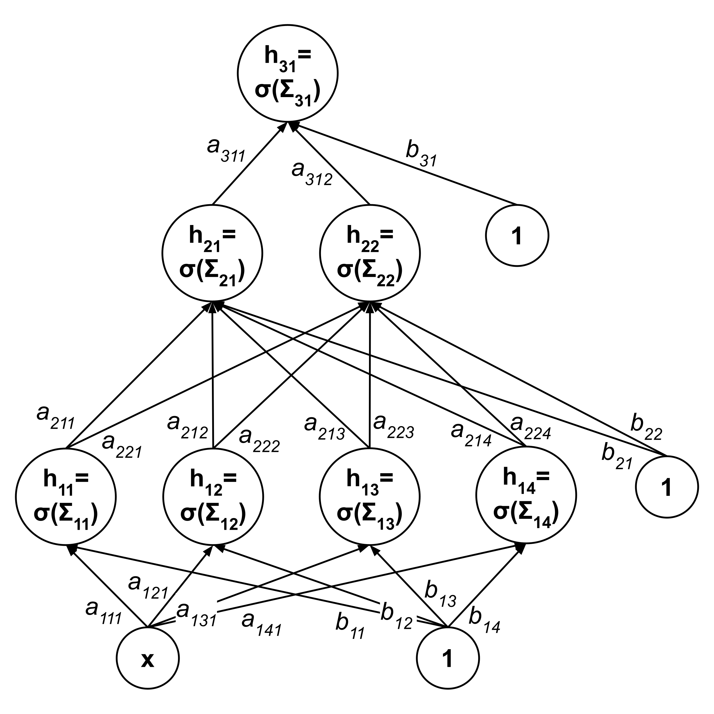
Now, let’s walk through an concrete example of fitting a neural network to a data set using the backpropagation algorithm. We will use the same data set and neural network architecture as the previous chapter:

$\begin{align*} \left[ (0,0), (0.25,1), (0.5,0.5), (0.75,1), (1,0) \right] \end{align*}$

Because neural networks are hierarchical and high-dimensional (i.e. they have many parameters that are tightly coupled), they are vastly more difficult to train as compared to simpler non-hierarchical low-dimensional models like linear, logistic, and polynomial regressions. Various tricks are often required to prevent the neural network from getting “stuck” in suboptimal local minima, which we will not cover here.

To provide a simple example that illustrates the training of a neural network to a high degree of accuracy while avoiding the need for more advanced tricks, we will intentionally choose the initial weights of our network to be similar to the weights that we arrived at when manually constructing a neural network in the previous chapter. (More specifically, they will be proportional by a factor of $0.5.$) This will place us near a deep valley on the surface of RSS as a function of parameters of the neural network, and the proximity will allow elementary gradient descent to lead us down into the valley.

So, we will use the following initial weights:

$\begin{align*} &A_1 = \begin{bmatrix} 5 \\ -5 \\ 5 \\ -5 \end{bmatrix} &&\vec b_1 = \begin{bmatrix} -0.75 \\ 1.75 \\ -3.25 \\ 4.25 \end{bmatrix} \\ \\ &A_2 = \begin{bmatrix} 10 & 10 & 0 & 0 \\ 0 & 0 & 10 & 10 \end{bmatrix} &&\vec b_2 = \begin{bmatrix} -12.5 \\ -12.5 \end{bmatrix} \\ \\ &A_3 = \begin{bmatrix} 10 & 10 \end{bmatrix} && \vec b_3 = \begin{bmatrix} -2.5 \end{bmatrix} \end{align*}$

Let’s work out the first iteration of backpropagation by hand, using learning rate $\alpha = 0.01.$ Note that the values shown are rounded to $6$ decimal places, but intermediate values are not actually rounded in the implementation.

Point: $(\vec x, y) = ([0],0)$

Forward propagation

$\begin{align*} \vec \Sigma_0 &= \vec x = \begin{bmatrix} 0 \end{bmatrix} \\[3pt] \vec h_0 &= \vec x = \begin{bmatrix} 0 \end{bmatrix} \\[10pt] \vec \Sigma_1 &= A_1 \vec h_0 + \vec b_1 = \begin{bmatrix} 5 \\ -5 \\ 5 \\ -5 \end{bmatrix} \begin{bmatrix} 0 \end{bmatrix}+ \begin{bmatrix} -0.75 \\ 1.75 \\ -3.25 \\ 4.25 \end{bmatrix} = \begin{bmatrix} -0.75 \\ 1.75 \\ -3.25 \\ 4.25 \end{bmatrix} \\[3pt] \vec h_1 &= \sigma \left( \vec \Sigma_1 \right) = \sigma \left( \begin{bmatrix} -0.75 \\ 1.75 \\ -3.25 \\ 4.25 \end{bmatrix} \right) = \begin{bmatrix} 0.320821 \\ 0.851953 \\ 0.037327 \\ 0.985936 \end{bmatrix} \\[10pt] \vec \Sigma_2 &= A_2 \vec h_1 + \vec b_2 = \begin{bmatrix} 10 & 10 & 0 & 0 \\ 0 & 0 & 10 & 10 \end{bmatrix} \begin{bmatrix} 0.320821 \\ 0.851953 \\ 0.037327 \\ 0.985936 \end{bmatrix} + \begin{bmatrix} -12.5 \\ -12.5 \end{bmatrix} = \begin{bmatrix} -0.772259 \\ -2.267367 \end{bmatrix} \\[3pt] \vec h_2 &= \sigma \left( \vec \Sigma_2 \right) = \sigma \left( \begin{bmatrix} -0.772259 \\ -2.267367 \end{bmatrix} \right) = \begin{bmatrix} 0.315991 \\ 0.093862 \end{bmatrix} \\[10pt] \vec \Sigma_3 &= A_3 \vec h_2 + \vec b_3 = \begin{bmatrix} 10 & 10 \end{bmatrix} \begin{bmatrix} 0.315991 \\ 0.093862 \end{bmatrix} + \begin{bmatrix} -2.5 \end{bmatrix} = \begin{bmatrix} 1.59852529 \end{bmatrix}\\[3pt] \vec h_3 &= \sigma \left( \vec \Sigma_3 \right) = \sigma \left( \begin{bmatrix} 1.598525 \end{bmatrix} \right) = \begin{bmatrix} 0.831812 \end{bmatrix} \end{align*}$

Backpropagation

$\begin{align*} \dfrac{\partial \textrm{RSS}}{\partial h_{31}} &= 2 \left( h_{31} - y \right) = 2 \left( 0.831812 - 0 \right) = 1.663624 \\[5pt] \dfrac{\partial \textrm{RSS}}{\partial \vec h_{2}} &= A_{3}^T \left( \dfrac{\partial \textrm{RSS}}{\partial \vec h_{3}} \circ \sigma' \left( \vec \Sigma_{3} \right) \right) = \begin{bmatrix} 10 \\ 10 \end{bmatrix} \left( \begin{bmatrix} 1.663624 \end{bmatrix} \circ \sigma' \left( \begin{bmatrix} 1.59852529 \end{bmatrix} \right) \right) = \begin{bmatrix} 2.327422 \\ 2.327422 \end{bmatrix} \\[5pt] \dfrac{\partial \textrm{RSS}}{\partial \vec h_{1}} &= A_{2}^T \left( \dfrac{\partial \textrm{RSS}}{\partial \vec h_{2}} \circ \sigma' \left( \vec \Sigma_{2} \right) \right) = \begin{bmatrix} 10 & 0 \\ 10 & 0 \\ 0 & 10 \\ 0 & 10 \end{bmatrix} \left( \begin{bmatrix} 2.327422 \\ 2.327422 \end{bmatrix} \circ \sigma' \left( \begin{bmatrix} -0.772259 \\ -2.267367 \end{bmatrix} \right) \right) = \begin{bmatrix} 5.030502 \\ 5.030502 \\ 1.979515 \\ 1.979515 \end{bmatrix} \end{align*}$

Expansion

$\begin{align*} \left. \dfrac{\partial \textrm{RSS}}{\partial \vec b_{3}} \right|_{([0], 0)} &= \dfrac{\partial \textrm{RSS}}{\partial \vec h_{3}} \circ \sigma' \left( \vec \Sigma_{3} \right) = \begin{bmatrix} 1.663624 \end{bmatrix} \circ \sigma' \left( \begin{bmatrix} 1.598525 \end{bmatrix} \right) = \begin{bmatrix} 0.232742 \end{bmatrix} \\[3pt] \left. \dfrac{\partial \textrm{RSS}}{\partial A_{3}} \right|_{([0], 0)} &= \left. \dfrac{\partial \textrm{RSS}}{\partial \vec b_{3}} \right|_{([0], 0)} \otimes \vec h_{2} = \begin{bmatrix} -0.000913 \end{bmatrix} \otimes \begin{bmatrix} 0.315991 \\ 0.093862 \end{bmatrix} = \begin{bmatrix} 0.073544 & 0.021846 \end{bmatrix} \\[10pt] \left. \dfrac{\partial \textrm{RSS}}{\partial \vec b_{2}} \right|_{([0], 0)} &= \dfrac{\partial \textrm{RSS}}{\partial \vec h_{2}} \circ \sigma' \left( \vec \Sigma_{2} \right) = \begin{bmatrix} 2.327422 \\ 2.327422 \end{bmatrix} \circ \sigma' \left( \begin{bmatrix} -0.772259 \\ -2.267367 \end{bmatrix} \right) = \begin{bmatrix} 0.503050 \\ 0.197951 \end{bmatrix} \\[3pt] \left. \dfrac{\partial \textrm{RSS}}{\partial A_{2}} \right|_{([0], 0)} &= \left. \dfrac{\partial \textrm{RSS}}{\partial \vec b_{2}} \right|_{([0], 0)} \otimes \vec h_{1} = \begin{bmatrix} 0.503050 \\ 0.197951 \end{bmatrix} \otimes \begin{bmatrix} 0.320821 \\ 0.851953 \\ 0.037327 \\ 0.985936 \end{bmatrix} = \begin{bmatrix} 0.161389 & 0.428575 & 0.018777 & 0.495976 \\ 0.063507 & 0.168645 & 0.007389 & 0.195168 \end{bmatrix} \\[10pt] \left. \dfrac{\partial \textrm{RSS}}{\partial \vec b_{1}} \right|_{([0], 0)} &= \dfrac{\partial \textrm{RSS}}{\partial \vec h_{1}} \circ \sigma' \left( \vec \Sigma_{1} \right) = \begin{bmatrix} 5.030502 \\ 5.030502 \\ 1.979515 \\ 1.979515 \end{bmatrix} \circ \sigma' \left( \begin{bmatrix} -0.75 \\ 1.75 \\ -3.25 \\ 4.25 \end{bmatrix} \right) = \begin{bmatrix} 1.096121 \\ 0.634493 \\ 0.071131 \\ 0.027448 \end{bmatrix} \\[3pt] \left. \dfrac{\partial \textrm{RSS}}{\partial A_{1}} \right|_{([0], 0)} &= \left. \dfrac{\partial \textrm{RSS}}{\partial \vec b_{1}} \right|_{([0], 0)} \otimes \vec h_{0} = \begin{bmatrix} 1.096121 \\ 0.634493 \\ 0.071131 \\ 0.027448 \end{bmatrix} \otimes \begin{bmatrix} 0 \end{bmatrix} = \begin{bmatrix} 0 \\ 0 \\ 0 \\ 0 \end{bmatrix} \end{align*}$

Point: $(\vec x, y) = ([0.25],1)$

$\begin{align*} &\vec \Sigma_0 = \begin{bmatrix} 0.25 \end{bmatrix} &&\vec h_0 = \begin{bmatrix} 0.25 \end{bmatrix} \\ \\ &\vec \Sigma_1 = \begin{bmatrix} 0.5 \\ 0.5 \\ -2 \\ 3 \end{bmatrix} &&\vec h_1 = \begin{bmatrix} 0.622459 \\ 0.622459 \\ 0.119203 \\ 0.952574 \end{bmatrix} \\ \\ &\vec \Sigma_2 = \begin{bmatrix} -0.050813 \\ -1.782230 \end{bmatrix} &&\vec h_2 = \begin{bmatrix} 0.487299 \\ 0.144028 \end{bmatrix} \\ \\ &\vec \Sigma_3 = \begin{bmatrix} 3.813274 \end{bmatrix} &&\vec h_3 = \begin{bmatrix} 0.978401 \end{bmatrix} \end{align*}$

$\begin{align*} \dfrac{\partial \textrm{RSS}}{\partial \vec h_{3}} = \begin{bmatrix} -0.043198 \end{bmatrix}, \quad \dfrac{\partial \textrm{RSS}}{\partial \vec h_{2}} = \begin{bmatrix} -0.009129 \\ -0.009129 \end{bmatrix}, \quad \dfrac{\partial \textrm{RSS}}{\partial \vec h_{1}} = \begin{bmatrix} -0.022807 \\ -0.022807 \\ -0.011254 \\ -0.011254 \end{bmatrix} \end{align*}$

$\begin{align*} &\left. \dfrac{\partial \textrm{RSS}}{\partial \vec b_{3}} \right|_{([0.25],1)} = \begin{bmatrix} -0.000913 \end{bmatrix} &&\left. \dfrac{\partial \textrm{RSS}}{\partial A_{3}} \right|_{([0.25],1)} = \begin{bmatrix} -0.000445 & -0.000131 \end{bmatrix} \\ \\ &\left. \dfrac{\partial \textrm{RSS}}{\partial \vec b_{2}} \right|_{([0.25],1)} = \begin{bmatrix} -0.002281 \\ -0.001125\end{bmatrix} &&\left. \dfrac{\partial \textrm{RSS}}{\partial A_{2}} \right|_{([0.25],1)} = \begin{bmatrix} -0.001420 & -0.001420 & -0.000272 & -0.002173 \\ -0.000701 & -0.000701 & -0.000134 & -0.001072 \end{bmatrix} \\ \\ &\left. \dfrac{\partial \textrm{RSS}}{\partial \vec b_{1}} \right|_{([0.25],1)} = \begin{bmatrix} -0.005360 \\ -0.005360 \\ -0.001182 \\ -0.000508 \end{bmatrix} &&\left. \dfrac{\partial \textrm{RSS}}{\partial A_{1}} \right|_{([0.25],1)} = \begin{bmatrix} -0.001340 \\ -0.001340 \\ -0.000295 \\ -0.000127 \end{bmatrix} \end{align*}$

Point: $(\vec x, y) = ([0.5],0.5)$

$\begin{align*} &\left. \dfrac{\partial \textrm{RSS}}{\partial \vec b_{3}} \right|_{([0.5],0.5)} = \begin{bmatrix} 0.020099 \end{bmatrix} &&\left. \dfrac{\partial \textrm{RSS}}{\partial A_{3}} \right|_{([0.5],0.5)} = \begin{bmatrix} 0.006351 & 0.006351 \end{bmatrix} \\ \\ &\left. \dfrac{\partial \textrm{RSS}}{\partial \vec b_{2}} \right|_{([0.5],0.5)} = \begin{bmatrix} 0.043443 \\ 0.043443 \end{bmatrix} &&\left. \dfrac{\partial \textrm{RSS}}{\partial A_{2}} \right|_{([0.5],0.5)} = \begin{bmatrix} 0.037011 & 0.013937 & 0.013937 & 0.037011 \\ 0.037011 & 0.013937 & 0.013937 & 0.037011 \end{bmatrix} \\ \\ &\left. \dfrac{\partial \textrm{RSS}}{\partial \vec b_{1}} \right|_{([0.5],0.5)} = \begin{bmatrix} 0.054794 \\ 0.094659 \\ 0.094659 \\ 0.054794 \end{bmatrix} &&\left. \dfrac{\partial \textrm{RSS}}{\partial A_{1}} \right|_{([0.5],0.5)} = \begin{bmatrix} 0.027397 \\ 0.047330 \\ 0.047330 \\ 0.027397 \end{bmatrix} \end{align*}$

Point: $(\vec x, y) = ([0.75],1)$

$\begin{align*} &\left. \dfrac{\partial \textrm{RSS}}{\partial \vec b_{3}} \right|_{([0.75],1)} = \begin{bmatrix} -0.000913 \end{bmatrix} &&\left. \dfrac{\partial \textrm{RSS}}{\partial A_{3}} \right|_{([0.75],1)} = \begin{bmatrix} -0.000131 & -0.000445 \end{bmatrix} \\ \\ &\left. \dfrac{\partial \textrm{RSS}}{\partial \vec b_{2}} \right|_{([0.75],1)} = \begin{bmatrix} -0.001125 \\ -0.002281 \end{bmatrix} &&\left. \dfrac{\partial \textrm{RSS}}{\partial A_{2}} \right|_{([0.75],1)} = \begin{bmatrix} -0.001072 & -0.000134 & -0.000701 & -0.000701 \\ -0.002173 & -0.000272 & -0.001420 & -0.001420 \end{bmatrix} \\ \\ &\left. \dfrac{\partial \textrm{RSS}}{\partial \vec b_{1}} \right|_{([0.75],1)} = \begin{bmatrix} -0.000508 \\ -0.001182 \\ -0.005360 \\ -0.005360 \end{bmatrix} &&\left. \dfrac{\partial \textrm{RSS}}{\partial A_{1}} \right|_{([0.75],1)} = \begin{bmatrix} -0.000381 \\ -0.000886 \\ -0.004020 \\ -0.004020 \end{bmatrix} \end{align*}$

Point: $(\vec x, y) = ([1],0)$

$\begin{align*} &\left. \dfrac{\partial \textrm{RSS}}{\partial \vec b_{3}} \right|_{([1],0)} = \begin{bmatrix} 0.232742 \end{bmatrix} &&\left. \dfrac{\partial \textrm{RSS}}{\partial A_{3}} \right|_{([1],0)} = \begin{bmatrix} 0.021846 & 0.073544 \end{bmatrix} \\ \\ &\left. \dfrac{\partial \textrm{RSS}}{\partial \vec b_{2}} \right|_{([1],0)} = \begin{bmatrix} 0.197951 \\ 0.503050 \end{bmatrix} &&\left. \dfrac{\partial \textrm{RSS}}{\partial A_{2}} \right|_{([1],0)} = \begin{bmatrix} 0.195168 & 0.007389 & 0.168645 & 0.063507 \\ 0.495976 & 0.018777 & 0.428575 & 0.161389 \end{bmatrix} \\ \\ &\left. \dfrac{\partial \textrm{RSS}}{\partial \vec b_{1}} \right|_{([1],0)} = \begin{bmatrix} 0.027448 \\ 0.071131 \\ 0.634493 \\ 1.096121 \end{bmatrix} &&\left. \dfrac{\partial \textrm{RSS}}{\partial A_{1}} \right|_{([1],0)} = \begin{bmatrix} 0.027448 \\ 0.071131 \\ 0.634493 \\ 1.096121 \end{bmatrix} \end{align*}$

Weight Updates

Summing up all the gradients we computed, we get the following:

$\begin{align*} &\dfrac{\partial \textrm{RSS}}{\partial \vec b_{3}} = \begin{bmatrix} 0.483758 \end{bmatrix} &&\dfrac{\partial \textrm{RSS}}{\partial A_{3}} = \begin{bmatrix} 0.101165 && 0.101165 \end{bmatrix} \\ \\ &\dfrac{\partial \textrm{RSS}}{\partial \vec b_{2}} = \begin{bmatrix} 0.741038 \\ 0.741038 \end{bmatrix} &&\dfrac{\partial \textrm{RSS}}{\partial A_{2}} = \begin{bmatrix} 0.391076 & 0.448347 & 0.200388 & 0.593621 \\ 0.593621 & 0.200388 & 0.448347 & 0.391076 \end{bmatrix} \\ \\ &\dfrac{\partial \textrm{RSS}}{\partial \vec b_{1}} = \begin{bmatrix} 1.172495 \\ 0.793742 \\ 0.793742 \\ 1.172495 \end{bmatrix} &&\dfrac{\partial \textrm{RSS}}{\partial A_{1}} = \begin{bmatrix} 0.053123 \\ 0.116235 \\ 0.677508 \\ 1.119371 \end{bmatrix} \end{align*}$

Finally, applying the gradient descent updates $A_\ell \to A_\ell - \alpha \dfrac{\textrm{RSS}}{\partial A_{\ell}}$ and $\vec b_\ell \to \vec b_\ell - \alpha \dfrac{\textrm{RSS}}{\partial \vec b_{\ell}}$ with $\alpha = 0.01,$ we get the following updated weights:

$\begin{align*} &A_1 = \begin{bmatrix} 4.999469 \\ -5.001162 \\ 4.993225 \\ -5.011194 \end{bmatrix} &&\vec b_1 = \begin{bmatrix} -0.761725 \\ 1.742063 \\ -3.257937 \\ 4.238275 \end{bmatrix} \\ \\ &A_2 = \begin{bmatrix} 9.996089 & 9.995517 & -0.002004 & -0.005936 \\ -0.005936 & -0.002004 & 9.995517 & 9.996089 \end{bmatrix} &&\vec b_2 = \begin{bmatrix} -12.507410 \\ -12.507410 \end{bmatrix} \\ \\ &A_3 = \begin{bmatrix} 9.998988 & 9.998988 \end{bmatrix} && \vec b_3 = \begin{bmatrix} -2.504838 \end{bmatrix} \end{align*}$

Demonstration of Many Iterations

Repeating this procedure over and over, we get the following results. Note that the values shown are rounded to $3$ decimal places, but intermediate values are not actually rounded in the implementation.

Initial

$\textrm{RSS} \approx 1.614$
$\textrm{Predictions} \approx 0.832, 0.978, 0.979, 0.978, 0.832$
$(\textrm{Compare to} \phantom{\approx} 0,\phantom{.000} 1,\phantom{.000} 0.5,\phantom{00} 1,\phantom{.000} 0)\phantom{.000}$

After $1$ iteration

$\textrm{RSS} \approx 1.525$
$\textrm{Predictions} \approx 0.812, 0.973, 0.973, 0.972, 0.801$

$\begin{align*} &A_1 = \begin{bmatrix} 4.999 \\ -5.001 \\ 4.993 \\ -5.011 \end{bmatrix} &&\vec b_1 = \begin{bmatrix} -0.762 \\ 1.742 \\ -3.258 \\ 4.238 \end{bmatrix} \\ \\ &A_2 = \begin{bmatrix} 9.996 & 9.996 & -0.002 & -0.006 \\ -0.006 & -0.002 & 9.996 & 9.996 \end{bmatrix} &&\vec b_2 = \begin{bmatrix} -12.507 \\ -12.507 \end{bmatrix} \\ \\ &A_3 = \begin{bmatrix} 9.999 & 9.999 \end{bmatrix} && \vec b_3 = \begin{bmatrix} -2.505 \end{bmatrix} \end{align*}$

After $2$ iterations

$\textrm{RSS} \approx 1.426$
$\textrm{Predictions} \approx 0.789, 0.967, 0.965, 0.962, 0.765$

$\begin{align*} &A_1 \approx \begin{bmatrix} 4.999 \\ -5.002 \\ 4.986 \\ -5.023 \end{bmatrix} &&\vec b_1 \approx \begin{bmatrix} -0.774 \\ 1.734 \\ -3.267 \\ 4.226 \end{bmatrix} \\ \\ &A_2 \approx \begin{bmatrix} 9.992 & 9.991 & -0.004 & -0.012 \\ -0.012 & -0.004 & 9.991 & 9.992 \end{bmatrix} &&\vec b_2 \approx \begin{bmatrix} -12.515 \\ -12.515 \end{bmatrix} \\ \\ &A_3 \approx \begin{bmatrix} 9.998 & 9.998 \end{bmatrix} && \vec b_3 \approx \begin{bmatrix} -2.510 \end{bmatrix} \end{align*}$

After $3$ iterations

$\textrm{RSS} \approx 1.320$
$\textrm{Predictions} \approx 0.764, 0.959, 0.954, 0.949, 0.725$

$\begin{align*} &A_1 \approx \begin{bmatrix} 4.998 \\ -5.004 \\ 4.978 \\ -5.035 \end{bmatrix} &&\vec b_1 \approx \begin{bmatrix} -0.787 \\ 1.725 \\ -3.276 \\ 4.213 \end{bmatrix} \\ \\ &A_2 \approx \begin{bmatrix} 9.987 & 9.986 & -0.006 & -0.019 \\ -0.019 & -0.006 & 9.986 & 9.988 \end{bmatrix} &&\vec b_2 \approx \begin{bmatrix} -12.524 \\ -12.524 \end{bmatrix} \\ \\ &A_3 \approx \begin{bmatrix} 9.997 & 9.997 \end{bmatrix} && \vec b_3 \approx \begin{bmatrix} -2.516 \end{bmatrix} \end{align*}$

After $10$ iterations

$\textrm{RSS} \approx 0.730$
$\textrm{Predictions} \approx 0.571, 0.844, 0.816, 0.774, 0.478$

$\begin{align*} &A_1 \approx \begin{bmatrix} 4.992 \\ -5.015 \\ 4.933 \\ -5.101 \end{bmatrix} &&\vec b_1 \approx \begin{bmatrix} -0.873 \\ 1.66 \\ -3.331 \\ 4.142 \end{bmatrix} \\ \\ &A_2 \approx \begin{bmatrix} 9.957 & 9.953 & -0.022 & -0.064 \\ -0.058 & -0.022 & 9.958 & 9.959 \end{bmatrix} &&\vec b_2 \approx \begin{bmatrix} -12.58 \\ -12.575 \end{bmatrix} \\ \\ &A_3 \approx \begin{bmatrix} 9.99 & 9.991 \end{bmatrix} && \vec b_3 \approx \begin{bmatrix} -2.557 \end{bmatrix} \end{align*}$

After $100$ iterations

$\textrm{RSS} \approx 0.496$
$\textrm{Predictions} \approx 0.362, 0.694, 0.730, 0.698, 0.356$

$\begin{align*} &A_1 \approx \begin{bmatrix} 5.068 \\ -4.962 \\ 4.965 \\ -5.158 \end{bmatrix} &&\vec b_1 \approx \begin{bmatrix} -0.936 \\ 1.696 \\ -3.249 \\ 4.164 \end{bmatrix} \\ \\ &A_2 \approx \begin{bmatrix} 9.920 & 9.862 & -0.064 & -0.15 \\ -0.116 & -0.074 & 9.894 & 9.921 \end{bmatrix} &&\vec b_2 \approx \begin{bmatrix} -12.708 \\ -12.683 \end{bmatrix} \\ \\ &A_3 \approx \begin{bmatrix} 9.978 & 9.981 \end{bmatrix} && \vec b_3 \approx \begin{bmatrix} -2.735 \end{bmatrix} \end{align*}$

After $1\,000$ iterations

$\textrm{RSS} \approx 0.198$
$\textrm{Predictions} \approx 0.199, 0.788, 0.668, 0.788, 0.202$

$\begin{align*} &A_1 \approx \begin{bmatrix} 5.491 \\ -5.101 \\ 5.343 \\ -5.152 \end{bmatrix} &&\vec b_1 \approx \begin{bmatrix} -0.518 \\ 2.008 \\ -3.081 \\ 4.546 \end{bmatrix} \\ \\ &A_2 \approx \begin{bmatrix} 9.744 & 9.666 & -0.301 & -0.425 \\ -0.442 & -0.301 & 9.668 & 9.721 \end{bmatrix} &&\vec b_2 \approx \begin{bmatrix} -13.155 \\ -13.170 \end{bmatrix} \\ \\ &A_3 \approx \begin{bmatrix} 9.982 & 9.98 \end{bmatrix} && \vec b_3 \approx \begin{bmatrix} -3.596 \end{bmatrix} \end{align*}$

After $10\,000$ iterations

$\textrm{RSS} \approx 0.0239$
$\textrm{Predictions} \approx 0.068, 0.922, 0.517, 0.915, 0.075$

$\begin{align*} &A_1 \approx \begin{bmatrix} 6.96 \\ -6.033 \\ 6.632 \\ -5.806 \end{bmatrix} &&\vec b_1 \approx \begin{bmatrix} -0.279 \\ 2.766 \\ -3.307 \\ 5.478 \end{bmatrix} \\ \\ &A_2 \approx \begin{bmatrix} 9.88 & 9.555 & -0.835 & -0.865 \\ -0.932 & -0.806 & 9.647 & 9.781 \end{bmatrix} &&\vec b_2 \approx \begin{bmatrix} -13.763 \\ -13.804 \end{bmatrix} \\ \\ &A_3 \approx \begin{bmatrix} 10.515 & 10.542 \end{bmatrix} && \vec b_3 \approx \begin{bmatrix} -4.759 \end{bmatrix} \end{align*}$

After $100\,000$ iterations

$\textrm{RSS} \approx 0.0020$
$\textrm{Predictions} \approx 0.020, 0.979, 0.501, 0.976, 0.023$

$\begin{align*} &A_1 \approx \begin{bmatrix} 8.407 \\ -7.103 \\ 7.786 \\ -6.971 \end{bmatrix} &&\vec b_1 \approx \begin{bmatrix} -0.523 \\ 3.289 \\ -3.906 \\ 6.412 \end{bmatrix} \\ \\ &A_2 \approx \begin{bmatrix} 10.437 & 9.708 & -1.367 & -1.063 \\ -1.179 & -1.311 & 9.922 & 10.416 \end{bmatrix} &&\vec b_2 \approx \begin{bmatrix} -14.075 \\ -14.139 \end{bmatrix} \\ \\ &A_3 \approx \begin{bmatrix} 11.607 & 11.800 \end{bmatrix} && \vec b_3 \approx \begin{bmatrix} -5.433 \end{bmatrix} \end{align*}$

After $1\,000\,000$ iterations

$\textrm{RSS} \approx 0.0002$
$\textrm{Predictions} \approx 0.006, 0.993, 0.500, 0.993, 0.007$

$\begin{align*} &A_1 \approx \begin{bmatrix} 9.527 \\ -7.895 \\ 8.602 \\ -7.956 \end{bmatrix} &&\vec b_1 \approx \begin{bmatrix} -0.738 \\ 3.651 \\ -4.384 \\ 7.219 \end{bmatrix} \\ \\ &A_2 \approx \begin{bmatrix} 11.006 & 9.855 & -1.801 & -1.214 \\ -1.405 & -1.730 & 10.129 & 11.100 \end{bmatrix} &&\vec b_2 \approx \begin{bmatrix} -14.323 \\ -14.440 \end{bmatrix} \\ \\ &A_3 \approx \begin{bmatrix} 12.902 & 13.223 \end{bmatrix} && \vec b_3 \approx \begin{bmatrix} -6.178 \end{bmatrix} \end{align*}$

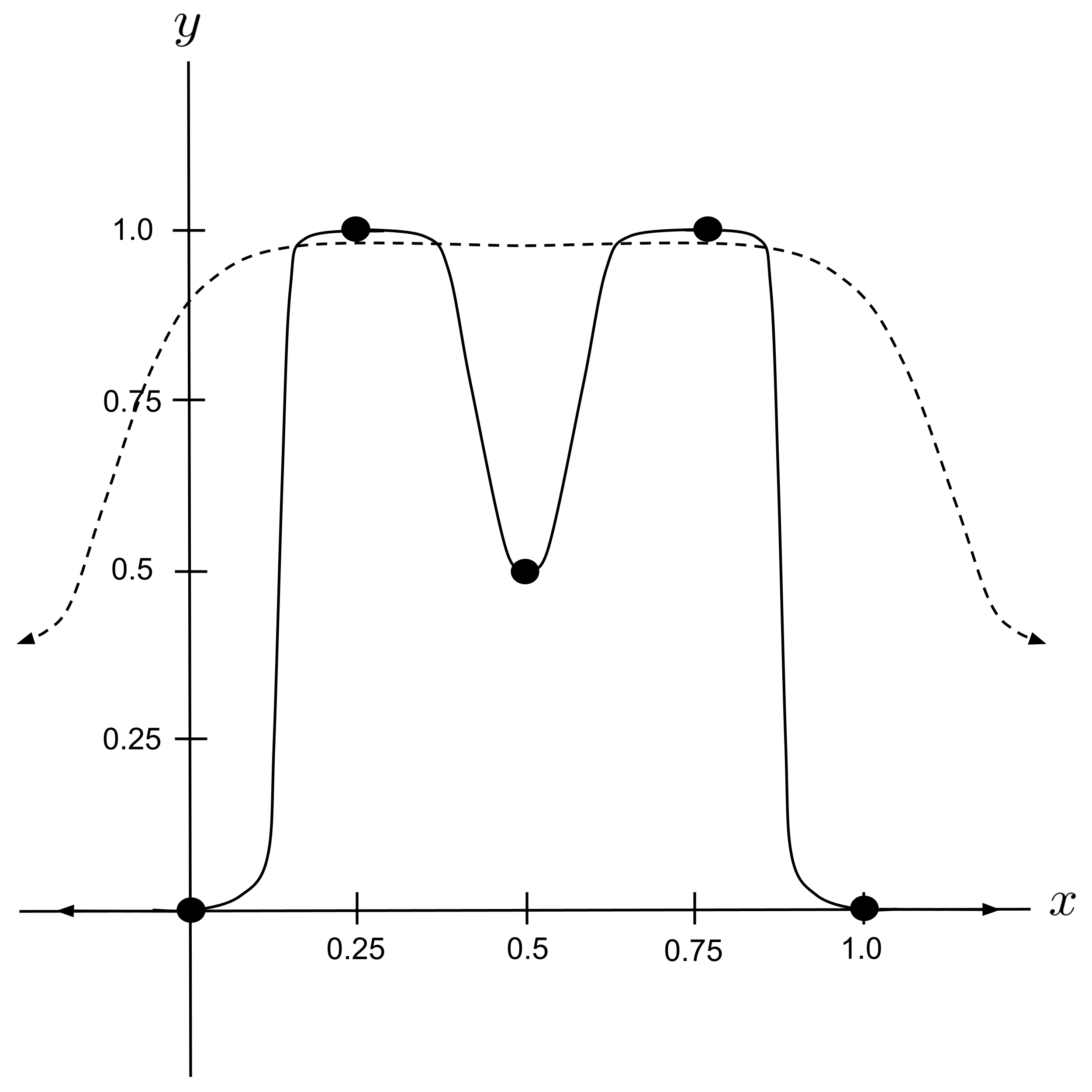
Below is a graph of the regression curves before and after training (i.e. using the initial weights and using the weights after $1\,000\,000$ iterations of backpropagation). The trained network does an even better job of passing through the leftmost and rightmost points than the network we constructed manually in the previous chapter!

Exercises

Implement the example that was worked out above.
Re-run the example that was worked out above, this time using initial weights drawn randomly from the normal distribution. Note that your RSS should gradually decrease but it may get "stuck" in a suboptimal local minimum, resulting in a regression curve that is a decent but not perfect fit.