Subtle Things to Watch Out For When Demonstrating Lp-Norm Regularization on a High-Degree Polynomial Regression Model
Initial parameter range, data sampling range, severity of regularization.
Want to get notified about new posts? Join the mailing list and follow on X/Twitter.
Background
This is something of a technical diary entry. I introduced a student to the idea of Lp regularization today. It came up naturally in discussion, and I hadn’t planned out anything beforehand, but I figured it shouldn’t be too hard to guide the student in throwing together a quick script to demonstrate the phenomenon.
The student had previously written a script to
- sample some data points from the stochastic process $f(x)=-2x^2+2x+\epsilon$ (where $\epsilon \sim U[-0.05, 0.05]$) over the interval $x \in [0,1],$ and then
- fit a general quadratic curve $p_2(x)=\beta_2 x^2 + \beta_1 x + \beta_0$ to that data using gradient descent (with initial parameters $\beta_i \sim U[-0.5, 0.5]$).
(Yes, you are guaranteed an optimal fit using the pseudoinverse, but we had already done that and were using the same setting as a simple introductory context for gradient descent. I also realize that noise and initial parameters are usually taken to be normally distributed, but the point of this exercise was to stay as simple as possible, so we ended up just using the uniform distribution. For pedagogical purposes it doesn’t really matter.)
So, I figured we could demonstrate the utility of regularization by doing the following:
- fit a high-degree (e.g., $9$th-degree) polynomial $p_n(x)=\beta_n x^n + \cdots + \beta_1 x + \beta_0$
- get an obviously overfitted (excessively curvy) result
- add an L2 regularization term $+ \lambda \sum_i \beta_i^2$ to the MSE loss function
- re-fit the high-degree polynomial and get a nice, smooth fit that looks more like a parabola
Resolving Issues
Extending the script to do this was easy enough. However, we ran into an issue where the high-degree polynomial looked like a fairly smooth parabolic fit from the outset (without any L2 regularization) and the L2 regularization just caused it to underfit (the curve essentially got “squashed” or vertically compressed, with the peak no longer as high as the corresponding peak in the data).
It took a bit of time to debug this experiment. There were three surprisingly subtle things that we needed to change in order to achieve the desired demonstration.
1. We had to expand the range for our initial parameters to something like $\beta_i \sim U[-20, 20]$ instead of $\beta_i \sim U[-20, 20].$ Our initial range $[-0.5, 0.5]$ was so small that it was still “implicitly” regularizing our polynomial, encouraging the initial parameters to be really small and therefore biasing the polynomial against curvature from the outset. After opening up that range to $[-20, 20],$ the polynomial was allowed to start off with plenty of curvature in its initial shape, which was then retained during the fitting procedure.
2. We had to narrow the sampling range to something like $x \in [0.3, 0.7]$ instead of $x \in [0, 1].$ In our initial sampling range $x \in [0,1],$ the loss function was being dominated by errors of points near $x \approx 1,$ so the fitting procedure was encouraged to pay much more attention to refining the polynomial’s fit around $x \approx 1$ than around $x \approx 0.$ (This was apparent in the polynomial’s shape: it would start get a bit excessively wavy on the far right, $x \in [0.8, 1],$ but looked very reasonably parabolic for the remainder of the range, $x \in [0, 0.8]$).
By shrinking the range and shifting it a bit to the right, the fitting procedure paid more equal attention across the entire range of $x$-values. (Of course, it still paid more attention to $x\approx 0.7$ than to $x \approx 0.3,$ but this difference in attention was not nearly as big as it would be between, say, $x \approx 0$ and $x \approx 0.4,$ which is in turn not nearly as the difference in attention between $x \approx 0$ and $x \approx 1.$)
3. We had to loosen up the severity of the regularization a bit, decreasing the regularization weight $\lambda.$ Originally, we were using $\lambda = 0.001$ which “looked” pretty small compared to all the other numbers that we were dealing with, but this was actually too severe to the point of overly constraining the polynomial. We lowered it down by one or two orders of magnitude and explored the range $\lambda \in [0.00001, 0.0001]$ with far better results.
Successful Results
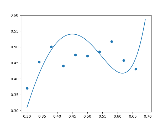
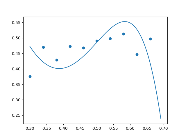
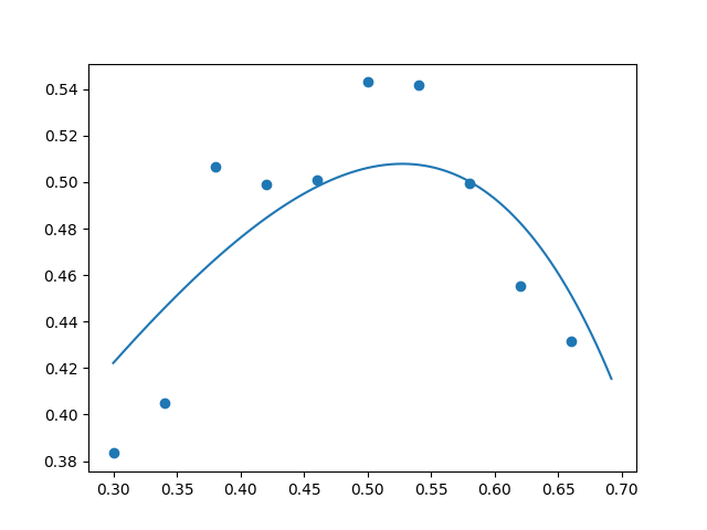
After making these tweaks, we saw excessive curvature in the unregularized $(\lambda = 0)$ polynomial, as desired. Below are some examples. The true data is along the parabola $y=-2x^2+2x$ with additive random noise uniformly sampled from the range $[-0.05, 0.05].$ We can see that the high-degree polynomial is going a bit crazy and fitting a peak and a valley when there is really just a peak (no valley) in the true underlying function $y=-2x^2+2x.$ (The high-degree polynomial is a bit paranoid and incorrectly thinks that the random noise in the data indicates the presence of multiple curves.)
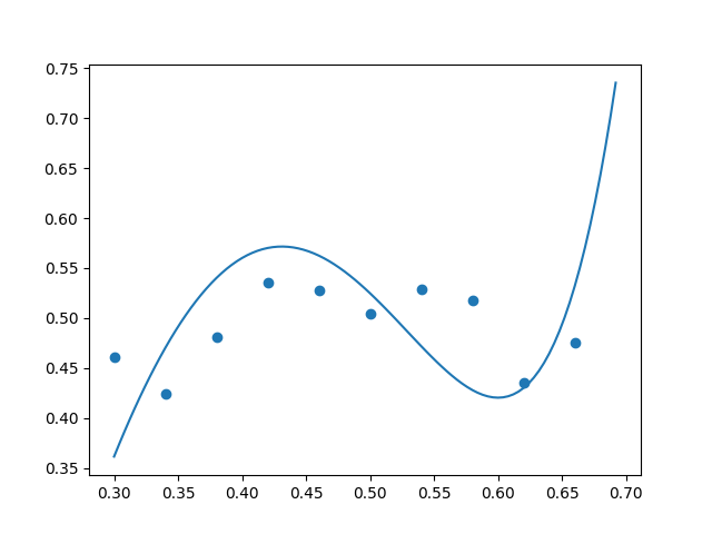
Using regularization coefficient $\lambda = 0.00001,$ we achieved “just enough” regularization:
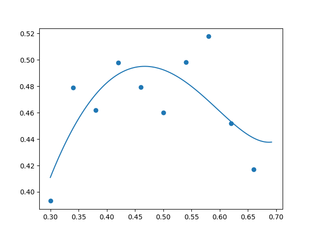
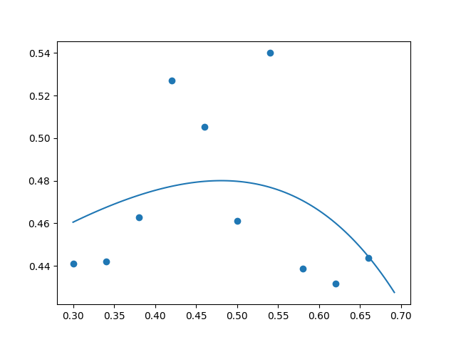
Increasing the coefficient to $\lambda = 0.00005,$ the result still looked pretty good (though perhaps bordering on a bit too much regularization):
But increasing the coefficient to $\lambda = 0.0001$ crossed the line into the territory of excessive regularization:
Want to get notified about new posts? Join the mailing list and follow on X/Twitter.