Slope Fields and Euler Approximation

When faced with a differential equation that we don't know how to solve, we can sometimes still approximate the solution.

This post is a chapter in the book Justin Math: Calculus. Suggested citation: Skycak, J. (2019). Slope Fields and Euler Approximation. Justin Math: Calculus. https://justinmath.com/slope-fields-and-euler-approximation/

When faced with a differential equation that we don’t know how to solve, we can sometimes still approximate the solution by simpler methods. If we just want to get an idea of what the solutions of the differential equation look like on a graph, we can construct a slope field.

Slope Fields

A slope field consists of an array of line segments, each line segment angled so that it represents the slope at the corresponding point.

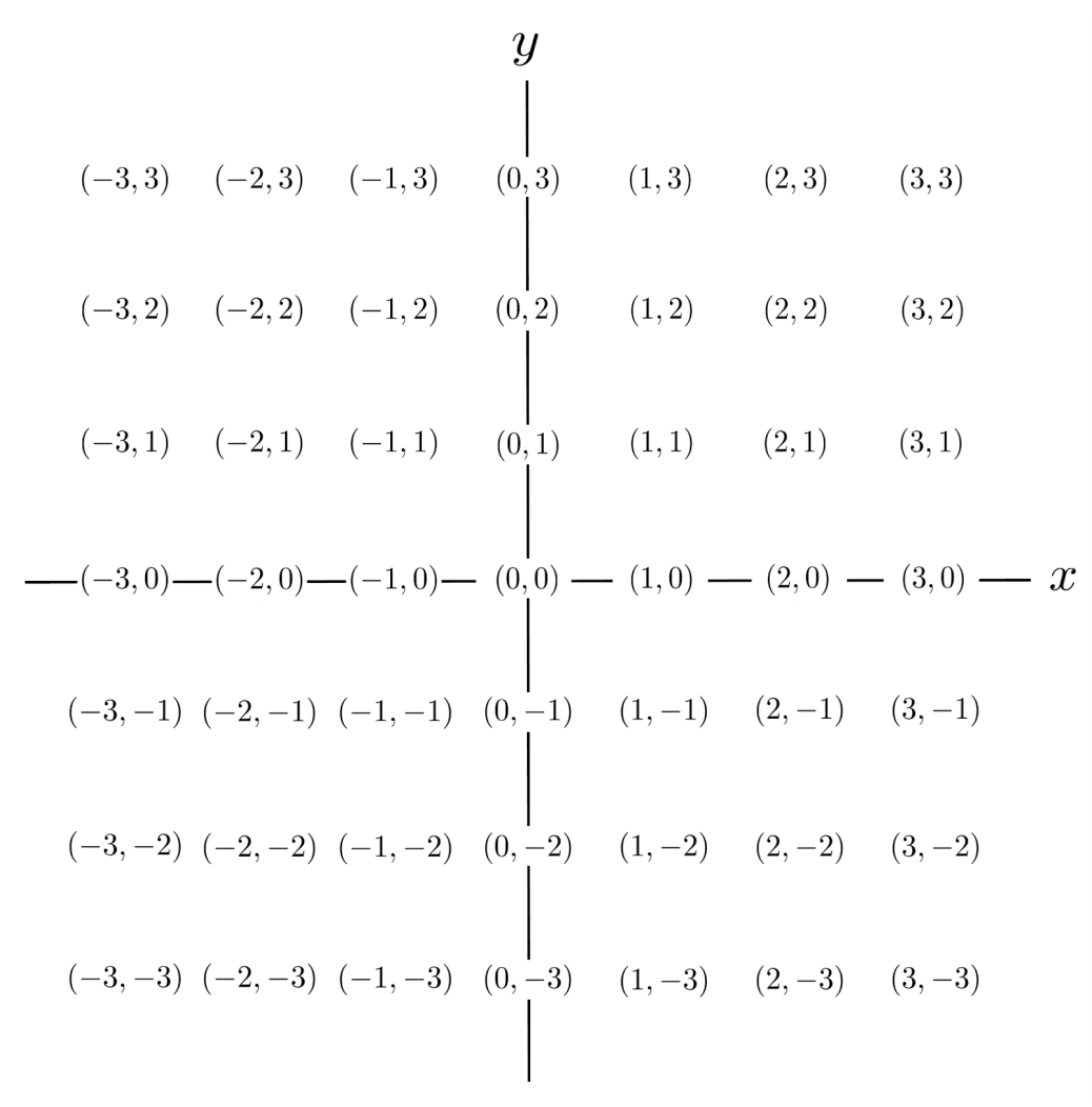
For example, to construct the slope field for the differential equation $y’=x^2-y$, we start with an array of points.

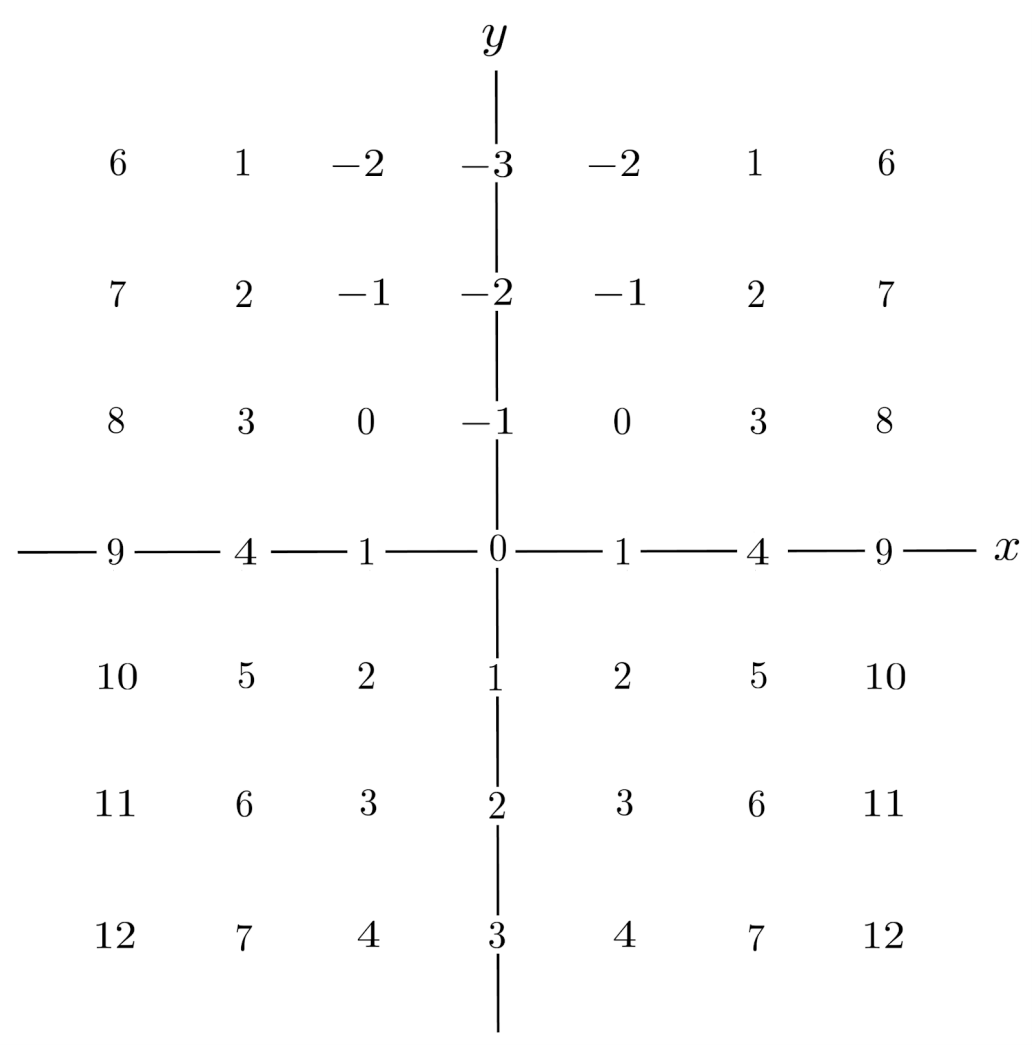
Then, we evaluate $y’$ at each point $(x,y)$.

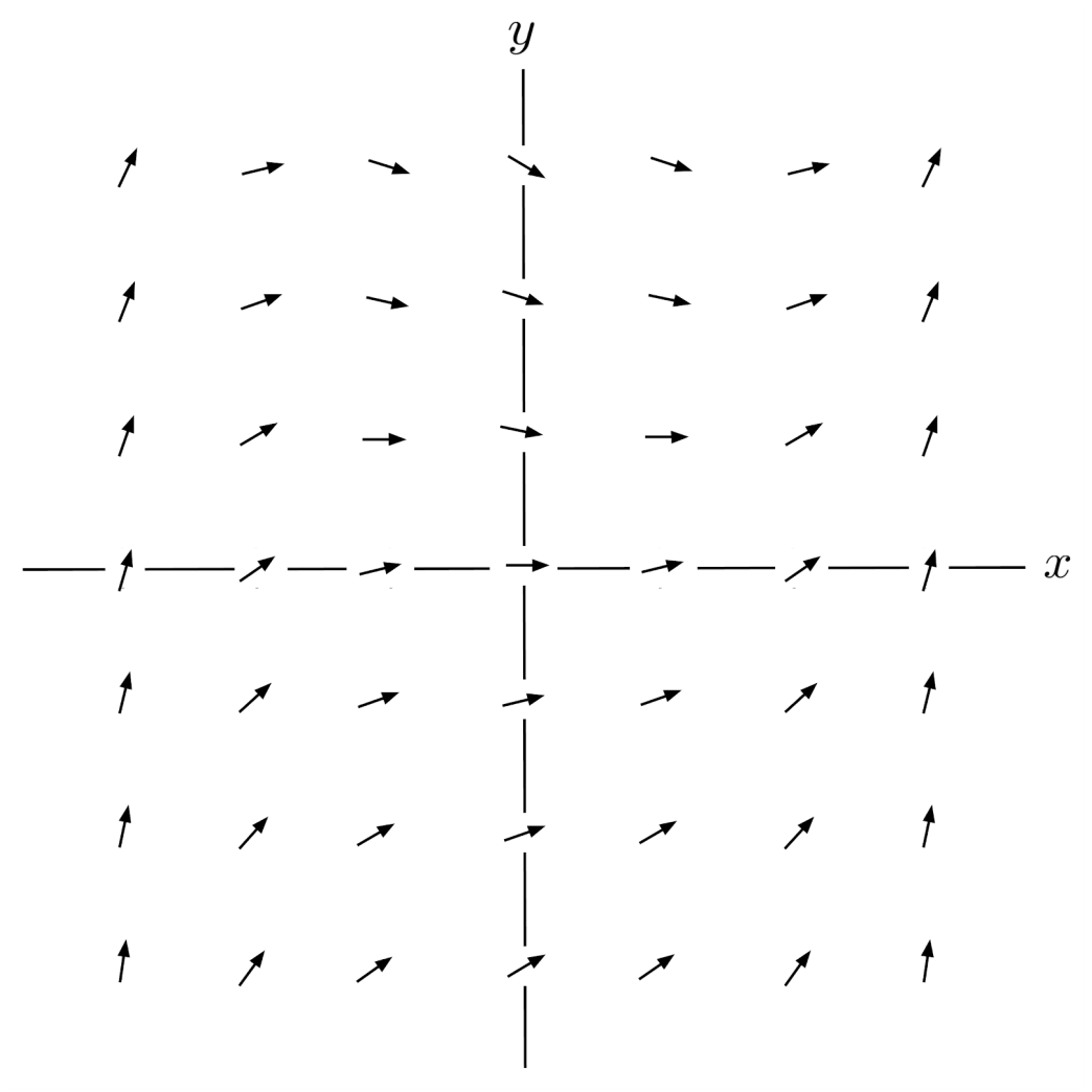
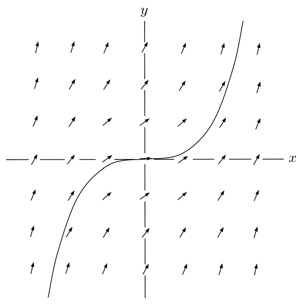
Lastly, we replace each value of $y’$ with a short arrow having that slope.

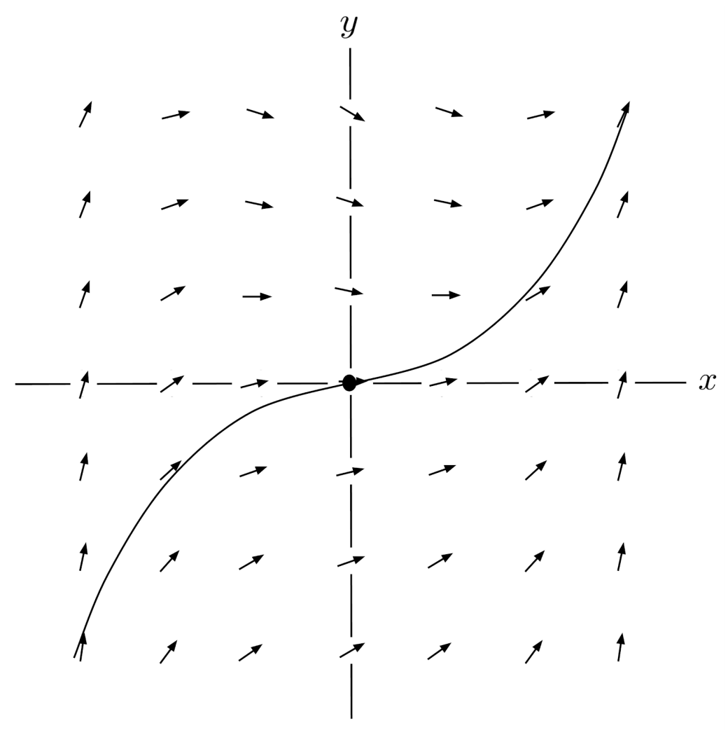
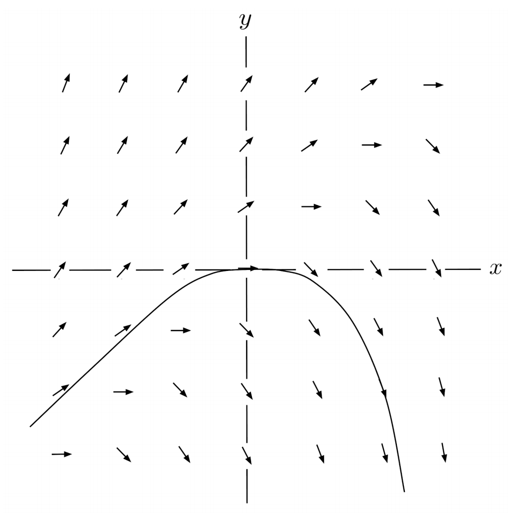
Now, we have an idea of what the solutions of the differential equation look like. For example, if we start at the point $(0,0)$ and follow the slopes as we go left and right, then we end up with the following curve.

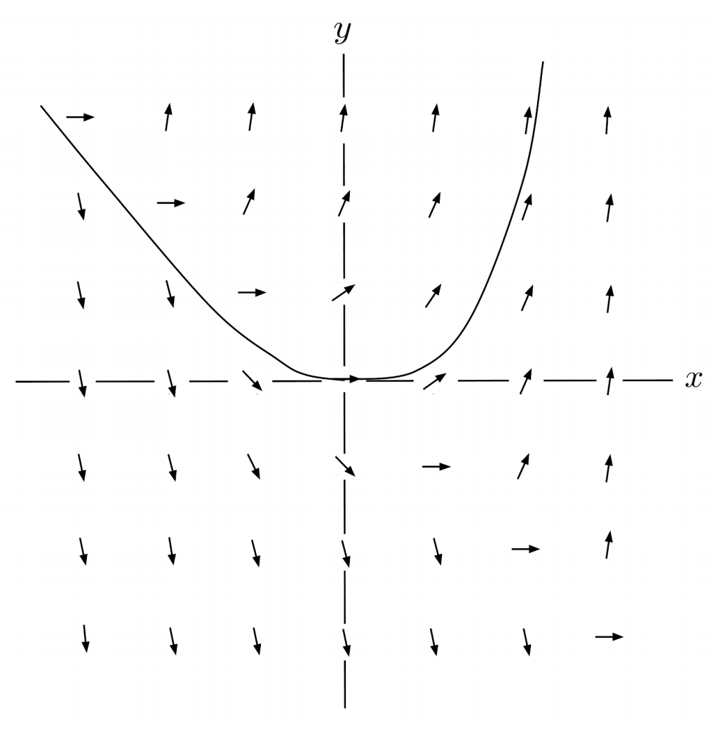
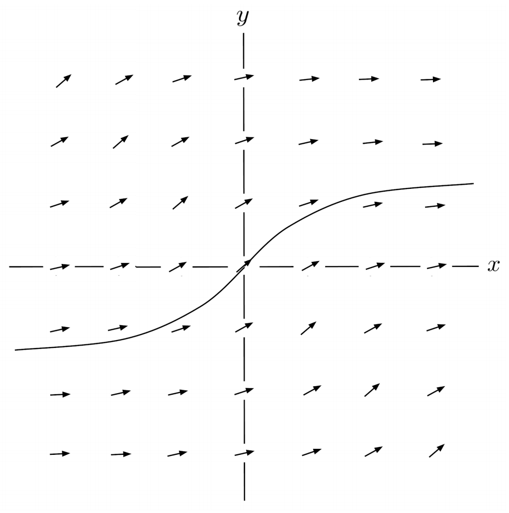
We can also choose a different point, say $(-2,2)$ to see the solution curve which contains that point.

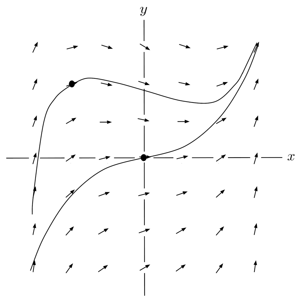
You can think of the coordinate plane as a river rapid, and the slope fields as the individual currents within the river rapid. If you launch a raft at a particular point, then the solution curve shows you where the river will take the raft.

Imprecision of Slope Fields

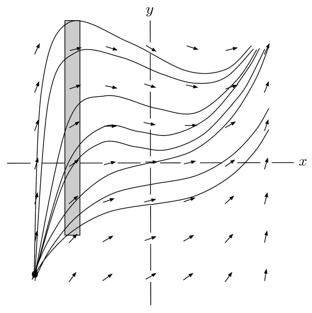
Although a slope field can show us the shapes of solutions to a differential equation, it isn’t very precise.

For example, if a particular solution starts at the point $(-3,-3)$, then the slope field tells us that it travels up and right – but exactly how far? If we travel right one units until the x-coordinate is $-2$, then what will the y-coordinate be?

Based on the sketch of the slope field, it’s hard to tell whether the y-coordinate will be closer to $-2$ or $4$. We need a more precise method.

Euler Estimation

We can estimate particular solutions more precisely using Euler approximation. In Euler approximation, we travel horizontally in small steps and use the derivative to compute how far we travel up or down at each step. The idea is that, since the solution curve is generated by this process with infinitesimally tiny step sizes, we can compute a good approximation to the solution curve if we use a small enough step size.

As an example, we will use Euler approximation to estimate the value of $y$ when $x=-2$, starting from the point $(-3,-3)$. We will use a step size of $\Delta x = 0.25$.

We start by computing $y’$ at the point $(-3,-3)$, using the differential equation $y’=x^2-y$, and obtaining a result of $(-3)^2-(-3)=12$.

Then, using $\Delta x = 0.25$, we estimate $\Delta y$ as $y’ \Delta x$, which is $(0.25)(12)=3$. We arrive at the point $(-3+0.25,-3+3)$, which simplifies to $(-2.75,0)$.

At this point, we compute the derivative again, use it and $\Delta x$ to estimate $\Delta y$, arrive at a new point, and continue the process until the x-coordinate is $-2$.

As shown in the table below, our resulting estimate of the y-coordinate is $3.5$.

Euler approximation tends to yield decent approximations for differential equations whose slope fields aren’t too turbulent, and the approximations can be made more accurate by decreasing the step size.

However, for differential equations that have singularities, one must be careful applying Euler approximation because it can “step over” asymptotes.

Exercises

Draw slope fields for the following differential equations on the grid $-3 \leq x, y \leq 3$.

Then, sketch a rough graph of the solution that passes through the point $(0,0)$.

Finally, starting at the point $(0,0)$, use Euler estimation with $4$ steps to approximate the value of $y$ when $x=1$. (Round to two decimal places throughout your calculations.)

(You can view the solution by clicking on the problem.)

$\begin{align*} 1) \hspace{.5cm} y' = y-x \end{align*}$

Solution:



$\begin{align*} y(0.25) &\approx 0 \\ y(0.5) &\approx -0.06 \\ y(0.75) &\approx -0.20 \\ y(1) &\approx -0.44 \end{align*}$

$\begin{align*} 2) \hspace{.5cm} y' = x^3 + y^3 \end{align*}$

Solution:



$\begin{align*} y(0.25) &\approx 0 \\ y(0.5) &\approx 0.01 \\ y(0.75) &\approx 0.04 \\ y(1) &\approx 0.15 \end{align*}$

$\begin{align*} 3) \hspace{.5cm} y' = \sqrt{x^2+y^2} \end{align*}$

Solution:



$\begin{align*} y(0.25) &\approx 0 \\ y(0.5) &\approx 0.06 \\ y(0.75) &\approx 0.19 \\ y(1) &\approx 0.38 \end{align*}$

$\begin{align*} 4) \hspace{.5cm} y'=\frac{1}{1+|x+y|} \end{align*}$

Solution:



$\begin{align*} y(0.25) &\approx 0.25 \\ y(0.5) &\approx 0.42 \\ y(0.75) &\approx 0.55 \\ y(1) &\approx 0.66 \end{align*}$

This post is a chapter in the book Justin Math: Calculus. Suggested citation: Skycak, J. (2019). Slope Fields and Euler Approximation. Justin Math: Calculus. https://justinmath.com/slope-fields-and-euler-approximation/