Shearing, Cramer’s Rule, and Volume by Reduction

by Justin Skycak on July 03, 2019

Shearing can be used to express the solution of a linear system using ratios of volumes, and also to compute volumes themselves.

This post is a chapter in the book Justin Math: Linear Algebra. Suggested citation: Skycak, J. (2019). Shearing, Cramer's Rule, and Volume by Reduction. Justin Math: Linear Algebra. https://justinmath.com/shearing-cramers-rule-and-volume-by-reduction/

Not only can a nonzero determinant tell us that a linear system has exactly one solution – the nonzero determinant can also help us quickly find that solution through a process known as Cramer’s rule.

Shearing

The key bit of intuition surrounding Cramer’s rule is the idea that moving one of the sides of a parallelepiped in a parallel direction does not change the volume of the parallelepiped. This kind of transformation is known as shearing, and the intuition can be most easily illustrated in 2 dimensions.

Suppose we have the following 2-dimensional linear system:

$\begin{align*} \begin{matrix} a_{11}x_1&+&a_{12}x_2&=& b_1 \\a_{21} x_1 & + & a_{22} x_2 &=& b_2 \end{matrix} \hspace{.5cm} \rightarrow \hspace{.5cm} x_1 \begin{pmatrix} a_{11} \\ a_{21} \end{pmatrix} + x_2 \begin{pmatrix} a_{12} \\ a_{22} \end{pmatrix} = \begin{pmatrix} b_1 \\ b_2 \end{pmatrix} \end{align*}$

The three vectors in this system – two coefficient vectors and one constant vector – can be represented visually as the vertices of a parallelogram.

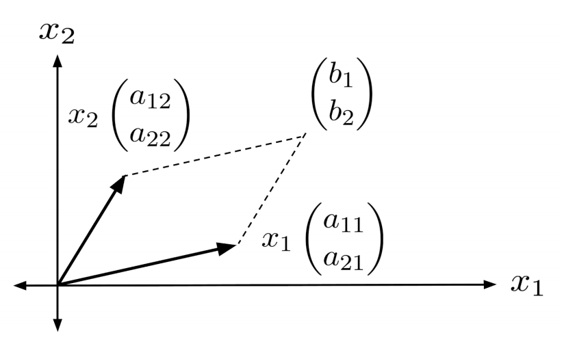
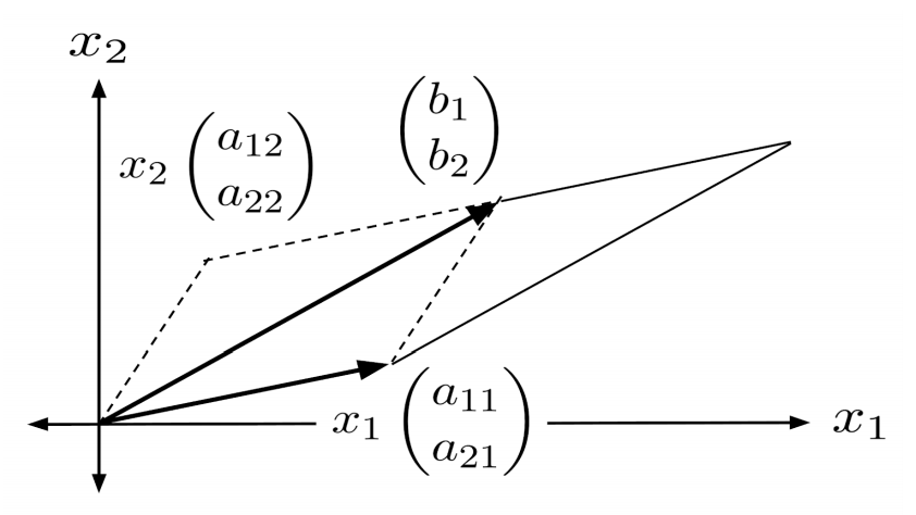
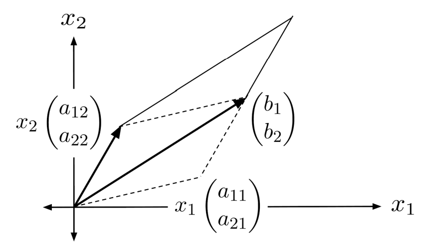
Notice that shearing the parallelogram does not change its area.

Cramer's Rule in Two Dimensions

Equating the volumes of the original parallelogram and the sheared parallelogram, we have

$\begin{align*} \det \begin{pmatrix} x_1 \begin{pmatrix} a_{11} \\ a_{21} \end{pmatrix}, x_2 \begin{pmatrix} a_{12} \\ a_{22} \end{pmatrix} \end{pmatrix} = \det \begin{pmatrix} x_1 \begin{pmatrix} a_{11} \\ a_{21} \end{pmatrix}, \begin{pmatrix} b_{1} \\ b_{2} \end{pmatrix} \end{pmatrix}. \end{align*}$

Using the fact that scaling a vector results in the volume being scaled by the same amount, we can simplify and solve for $x_2$.

$\begin{align*} x_1 x_2 \, \mbox{det} \begin{pmatrix} \begin{pmatrix} a_{11} \\ a_{21} \end{pmatrix}, \begin{pmatrix} a_{12} \\ a_{22} \end{pmatrix} \end{pmatrix} = x_1\, \mbox{det} \begin{pmatrix} \begin{pmatrix} a_{11} \\ a_{21} \end{pmatrix}, \begin{pmatrix} b_{1} \\ b_{2} \end{pmatrix} \end{pmatrix} \\ x_2 = \frac{ \mbox{det} \begin{pmatrix} \begin{pmatrix} a_{11} \\ a_{21} \end{pmatrix}, \begin{pmatrix} b_{1} \\ b_{2} \end{pmatrix} \end{pmatrix} }{ \mbox{det} \begin{pmatrix} \begin{pmatrix} a_{11} \\ a_{21} \end{pmatrix}, \begin{pmatrix} a_{12} \\ a_{22} \end{pmatrix} \end{pmatrix} } \end{align*}$

This is the solution for $x_2$ in the original system! We can use the same method to solve for $x_1$, too.

$\begin{align*} \mbox{det} \begin{pmatrix} x_1 \begin{pmatrix} a_{11} \\ a_{21} \end{pmatrix}, x_2 \begin{pmatrix} a_{12} \\ a_{22} \end{pmatrix} \end{pmatrix} = \mbox{det} \begin{pmatrix} \begin{pmatrix} b_{1} \\ b_{2} \end{pmatrix}, x_2 \begin{pmatrix} a_{12} \\ a_{22} \end{pmatrix} \end{pmatrix} \\ x_1 x_2 \, \mbox{det} \begin{pmatrix} \begin{pmatrix} a_{11} \\ a_{21} \end{pmatrix}, \begin{pmatrix} a_{12} \\ a_{22} \end{pmatrix} \end{pmatrix} = x_2 \, \mbox{det} \begin{pmatrix} \begin{pmatrix} b_{1} \\ b_{2} \end{pmatrix}, \begin{pmatrix} a_{12} \\ a_{22} \end{pmatrix} \end{pmatrix} \\ x_1 = \frac{ \mbox{det} \begin{pmatrix} \begin{pmatrix} b_{1} \\ b_{2} \end{pmatrix}, \begin{pmatrix} a_{12} \\ a_{22} \end{pmatrix} \end{pmatrix} }{ \mbox{det} \begin{pmatrix} \begin{pmatrix} a_{11} \\ a_{21} \end{pmatrix}, \begin{pmatrix} a_{12} \\ a_{22} \end{pmatrix} \end{pmatrix} } \end{align*}$

This method is known as Cramer’s rule. We illustrate it below on a concrete example, which would otherwise be annoying to solve by reduction because its solutions are fractional.

$\begin{align*} x_1 &= \frac{ \mbox{det} \begin{pmatrix} \begin{pmatrix} 7 \\ 4 \end{pmatrix}, \begin{pmatrix} -3 \\ 1 \end{pmatrix} \end{pmatrix} }{ \mbox{det} \begin{pmatrix} \begin{pmatrix} 2 \\ 5 \end{pmatrix}, \begin{pmatrix} -3 \\ 1 \end{pmatrix} \end{pmatrix} } = \frac{19}{17} \\ x_2 &= \frac{ \mbox{det} \begin{pmatrix} \begin{pmatrix} 2 \\ 5 \end{pmatrix}, \begin{pmatrix} 7 \\ 4 \end{pmatrix} \end{pmatrix} }{ \mbox{det} \begin{pmatrix} \begin{pmatrix} 2 \\ 5 \end{pmatrix}, \begin{pmatrix} -3 \\ 1 \end{pmatrix} \end{pmatrix} } = \frac{-27}{17} \end{align*}$

Cramer's Rule in N Dimensions

To generalize Cramer’s rule to N dimensions, we first come up with a compact notation for writing systems of linear equations.

$\begin{align*} &\begin{matrix} a_{11}x_1&+&a_{12}x_2&=& b_1 \\a_{21} x_1 & + & a_{22} x_2 &=& b_2 \end{matrix} \\ & \hspace{2cm} \downarrow \\ &\begin{pmatrix} a_{11} \\ a_{21} \end{pmatrix} x_1 + \begin{pmatrix} a_{12} \\ a_{22} \end{pmatrix} x_2 = \begin{pmatrix} b_1 \\ b_2 \end{pmatrix} \\ & \hspace{2cm} \downarrow \\ &a_1 x_1+ a_2 x_2 = b \end{align*}$

In this notation, we reduce the linear system to a single equation in terms of the vectors $a_1 = \left< a_{11}, a_{21} \right>$, $a_2 = \left< a_{12}, a_{22} \right>$, and $b=\left< b_1, b_2 \right>$. The solutions from Cramer’s rule can then be written as follows:

$\begin{align*} x_1 = \frac{\mbox{det}(b,a_2)}{\mbox{det}(a_1, a_2)} \hspace{1cm} x_2 = \frac{\mbox{det}(a_1,b)}{\mbox{det}(a_1, a_2)} \end{align*}$

The pattern is clear: $x_i$ is given by a fraction whose denominator is the determinant of the coefficient vectors, and whose numerator is the same except that the $i$th coefficient vector $a_i$ is replaced with the constant vector $b$.

For an N-dimensional square linear system, then, the solutions to

$\begin{align*} a_1 x_1 + a_2 x_2 + \ldots + a_n x_n = b \end{align*}$

are given by

$\begin{align*} x_i = \frac{\mbox{det}(a_1, \ldots, a_{i-1}, b, a_{i+1}, \ldots, a_n)}{\mbox{det}(a_1, a_2, \ldots, a_n)} \, . \end{align*}$

Volume by Reduction

Now, let’s take a step back and talk more about the elegance of shearing. We have seen that through Cramer’s rule, shearing can be used to express the solution of a linear system using ratios of volumes. Now, we will see that shearing can also be used to compute volumes themselves, without having to use the volume formula.

In a set of vectors, shearing simply amounts to adding one vector to another vector. Consequently, reducing a set of vectors preserves the volume of the parallelepiped formed by those vectors, provided that we don’t rescale any of the vectors themselves (otherwise, the volume would be rescaled as well).

The volume of a reduced set of vectors is much easier to compute: we can simply multiply the diagonal, because the diagonal entries are the parallelepiped’s lengths in each dimension.

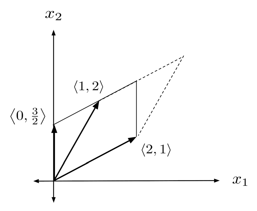
As a simple example, we can use shearing to compute the volume enclosed by the vectors $\left< 2,1 \right>$ and $\left< 1,2 \right>$.

$\begin{align*} \mbox{det} \begin{pmatrix} \left< 2,1 \right> \\ \left< 1,2 \right> \end{pmatrix} = \mbox{det} \begin{pmatrix} \left< 2,1 \right> \\ \left< 1,2 \right> - \frac{1}{2} \left< 2,1 \right> \end{pmatrix} = \mbox{det} \begin{pmatrix} \left< 2,1 \right> \\ \left< 0,\frac{3}{2} \right> \end{pmatrix} = 2 \cdot \frac{3}{2} = 3 \end{align*}$

When computing the volume of 4 or more vectors, it is much faster to use shearing instead of the volume formula. Below is an example of a 4-dimensional volume calculation using shearing.

$\begin{align*} \mbox{det} \begin{pmatrix} \left< 1,2,3,4 \right> \\ \left< 1,3,2,4 \right> \\ \left< 4,3,2,1 \right> \\ \left< 3,2,1,4 \right> \end{pmatrix} &= \mbox{det} \begin{pmatrix} \left< 1,2,3,4 \right> \\ \left< 1,3,2,4 \right> - \left< 1,2,3,4 \right> \\ \left< 4,3,2,1 \right> - 4\left< 1,2,3,4 \right> \\ \left< 3,2,1,4 \right> - 3\left< 1,2,3,4 \right> \end{pmatrix} \\ &= \mbox{det} \begin{pmatrix} \left< 1,2,3,4 \right> \\ \left< 0,1,-1,0 \right> \\ \left< 0,-5,-10,-15 \right>+5\left< 0,1,-1,0 \right> \\ \left< 0,-4,-8,-8 \right>+4\left< 0,1,-1,0 \right> \end{pmatrix} \\ &= \mbox{det} \begin{pmatrix} \left< 1,2,3,4 \right> \\ \left< 0,1,-1,0 \right> \\ \left< 0,0,-15,-15 \right> \\ \left< 0,0,-12,-8 \right> - \frac{12}{15} \left< 0,0,-15,-15 \right> \end{pmatrix} \\ &= \mbox{det} \begin{pmatrix} \left< 1,2,3,4 \right> \\ \left< 0,1,-1,0 \right> \\ \left< 0,0,-15,-15 \right> \\ \left< 0,0,0,4 \right> \end{pmatrix} \\ &= (1)(1)(-15)(4) \\ &= -60 \end{align*}$

Exercises

State whether the linear system has A) exactly one solution, or B) no solutions or infinitely many solutions. If there is A) exactly one solution, then use Cramer’s rule to find it.

In your calculations of determinants in higher than 3 dimensions, be sure to use the technique of shearing – it will save lots of time! (You can view the solution by clicking on the problem.)

$\begin{align*} 1) \hspace{.5cm} x+2y &= 4 \\ 2x-3y &= 3 \end{align*}$

Solution:
$\begin{align*} & \mbox{A) exactly one solution} \\ &x = \frac{18}{7} \\ &y = \frac{5}{7} \end{align*}$

$\begin{align*} 2) \hspace{.5cm} 3x+y &= -1 \\ x-2y &= 4 \end{align*}$

Solution:
$\begin{align*} & \mbox{A) exactly one solution} \\ &x = \frac{2}{7} \\ &y = -\frac{13}{7} \end{align*}$

$\begin{align*} 3) \hspace{.5cm} 5x+8y &= 2 \\ 3x-7y &= 5 \end{align*}$

Solution:
$\begin{align*} & \mbox{A) exactly one solution} \\ &x = \frac{54}{59} \\ &y= -\frac{19}{59} \end{align*}$

$\begin{align*} 4) \hspace{.5cm} 3x+7y &= 4 \\ 10x-6y &= -3 \end{align*}$

Solution:
$\begin{align*} & \mbox{A) exactly one solution} \\ &x = \frac{3}{88} \\ &y = \frac{49}{88} \end{align*}$

$\begin{align*} 5) \hspace{.5cm} x+2y+3z &= 8 \\ 2x+y-z &= 1 \\ x+y-z &= 2 \end{align*}$

Solution:
$\begin{align*} & \mbox{A) exactly one solution} \\ &x = -1 \\ &y = \frac{18}{5} \\ &z = \frac{3}{5} \end{align*}$

$\begin{align*} 6) \hspace{.5cm} 3x-y+z &= 1 \\ 6x + y + z &= 2 \\ 3y-z &= 3 \end{align*}$

Solution:
$\begin{align*} &\mbox{B) no solutions or} \\ &\mbox{infinitely many solutions} \end{align*}$

$\begin{align*} 7) \hspace{.5cm} x+2y-z &= 1 \\ 3x-3y+z &= 7 \\ -x+7y+z &= -3 \end{align*}$

Solution:
$\begin{align*} & \mbox{A) exactly one solution} \\ &x = \frac{35}{18} \\ &y = -\frac{2}{9} \\ &z = \frac{1}{2} \end{align*}$

$\begin{align*} 8) \hspace{.5cm} 4x-3y+2z &= 1 \\ 2x+3y+4z &= 1 \\ x-y+z &= 1 \end{align*}$

Solution:
$\begin{align*} & \mbox{A) exactly one solution} \\ &x=-\frac{5}{6} \\ &y= -\frac{2}{3} \\ &z = \frac{7}{6} \end{align*}$

$\begin{align*} 9) \hspace{.5cm} w+x+y+z &= 3 \\ w+y+z &= 2 \\ x+y+z &= -1 \\ 3w-4z &= 7 \end{align*}$

Solution:
$\begin{align*} & \mbox{A) exactly one solution} \\ &w=4 \\ &x = -\frac{13}{4} \\ &y=1 \\ &z = \frac{5}{4} \end{align*}$

$\begin{align*} 10) \hspace{.5cm} 4w+4x-y+z &= 4 \\ 2w-4x+y+z &= 3 \\ w+4x-y &= 3 \\ w+3x+y &= 1 \end{align*}$

Solution:
$\begin{align*} &\mbox{B) no solutions or} \\ &\mbox{infinitely many solutions} \end{align*}$

$\begin{align*} 11) \hspace{.5cm} u+3w+4x-y+z &= 1 \\ u-2w-4x+y+z &= -1 \\ 4u+4x-y &= 0 \\ w+2x-y &= 1 \\ 3w-x &= 2 \end{align*}$

Solution:
$\begin{align*} & \mbox{A) exactly one solution} \\ &u=\frac{1}{12} \\ &w= \frac{8}{15} \\ &x = -\frac{2}{5} \\ &y = -\frac{19}{15} \\ &z = -\frac{7}{20} \end{align*}$

$\begin{align*} 12) \hspace{.5cm} 3u-2w+x+y &= 0 \\ u-y-z &= 1 \\ w+x+y-3z &= 3 \\ u+2x+3z &= -2 \\ 2u-x+y-z &= -2 \end{align*}$

Solution:
$\begin{align*} & \mbox{A) exactly one solution} \\ &u=-\frac{11}{15} \\ &w=-\frac{13}{15} \\ &x= \frac{16}{15} \\ &y= -\frac{3}{5} \\ &z= -\frac{17}{15} \end{align*}$