Shaping STDP Neural Networks with Periodic Stimulation: a Theoretical Analysis for the Case of Tree Networks

by Justin Skycak (@justinskycak) on August 01, 2015

We solve a special case of how to periodically stimulate a biological neural network to obtain a desired connectivity (in theory).

Want to get notified about new posts? Join the mailing list and follow on X/Twitter.

We solve a special case of how to periodically stimulate a biological neural network undergoing spike-timing dependent plasticity to obtain a desired connectivity (in theory).

Model

We model neuronal networks as weighted directed graphs. Each vertex $i$ is a neuron having activity value $a_i(t) \in \lbrace 0, \delta(0) \rbrace$ at time $t,$ where $\delta$ is the Dirac delta function and represents an action potential or “spike.” Each edge $i \leftarrow j$ is a synapse in which neuron $i$ receives neurotransmitters from neuron $j,$ and the weight of the synapse at time $t$ is given by $w_{ij}(t).$ Neuron $j$ is said to be a neighbor of neuron $i$ if the weight of the synapse $w_{ij}(t)$ is nonzero.

A neuron becomes “excited” a duration of $\tau \approx 10$ ms [1] after a neighboring neuron spikes ($\tau$ is called the spike propagation latency). If it has been at least $r \approx 5$ ms since the neuron’s previous spike, then the excited neuron spikes ($r$ is called the refractory period). Otherwise, it does not. Formally, we have

$\begin{align*} a_i(t) = \begin{cases} \delta(0) & \mbox{if } a_i(t') = 0 \mbox{ for } t-r < t' < t \\[3pt] & \mbox{and } \exists j \in V \mbox{ such that } w_{ij}(t-\tau) > 0 \mbox{ and } a_j(t-\tau) = \delta(0) \\[3pt] 0 & \mbox{otherwise} \end{cases} \end{align*}$

The weights evolve over time according to the principles of weight decay and spike-timing dependent plasticity (STDP). Weight decay ensures that the weight of an unused synapse decays to zero. STDP is a biological neural learning rule where the weight is strengthened in a predictive fashion: if neuron $i$ spikes after neuron $j$ and the weight $w_{ij}$ is nonzero, then then the weight $w_{ij}$ increases and the weight $w_{ji}$ decreases. The smaller the time between the spikes of neurons $i$ and $j,$ the greater the magnitude of increase or decrease of the weight.

Let $s_i(t) = t - \min a_i^{-1} (\delta(0))$ be the time since neuron $i$ last spiked. The weights update according to

$\begin{align*} \frac{dw_{ij}}{dt} = f_{ij}(t) w_{ij}(t) \delta(0) \end{align*}$

where $f_{ij}(t)$ is the STDP function given by

$\begin{align*} f_{ij}(t) = \begin{cases} \alpha e^{-ks_j(t)} & \mbox{if } a_i(t) = \delta(0) \\[3pt] - \beta e^{-ks_i(t)} & \mbox{if } a_j(t) = \delta(0) \\[3pt] 0 & \mbox{otherwise}. \end{cases} \end{align*}$

In this STDP function, $k$ is on the order of $0.1 \textrm{ ms}^{-1}$ [2] and $\alpha, \beta \ll 1.$

We can also express the weight update as a multiplicative rule

$\begin{align*} w_{ij}(t+dt) &= w_{ij}(t) + w_{ij}(t)f_{ij}(t) \\[5pt] &= (1+f_{ij}(t)) w_{ij}(t). \end{align*}$

We ensure that there is not a bias towards increase or decrease of weights in the case of symmetric spike-timing differences by choosing $\alpha$ and $\beta$ such that

$\begin{align*} \left( 1 + \alpha e^{-ks_j(t)} \right) \left( 1-\beta e^{-ks_i(t)} \right) = 1. \end{align*}$

This is accomplished by choosing

$\begin{align*} \beta = \frac{\alpha}{1-\alpha \exp(-ks_i(t))}. \end{align*}$

With this choice, the STDP rule can be written as

$\begin{align*} f_{ij}(t) = \begin{cases} \frac{\alpha}{\exp(ks_j(t))} & \mbox{if } a_i(t) = \delta(0) \\[3pt] -\frac{\alpha}{\exp(ks_i(t))-\alpha} & \mbox{if } a_j(t) = \delta(0) \\[3pt] 0 & \mbox{otherwise}. \end{cases} \end{align*}$

In the following sections, we will investigate how periodic stimulation from an external source affects the connectivity of neuronal networks. We initialize weights as finite positive numbers, and we say that a weight

solidifies if it is asymptotically infinite, i.e. $\lim_{t \to \infty} w_{ij}(t) = \infty$;
breaks if it is asymptotically zero, i.e. $\lim_{t \to \infty} w_{ij}(t) = 0$; and
remains fluid if it is neither asymptotically infinite nor asymptotically zero.

Analysis

We first consider the case where a single neuron in a tree network experiences periodic stimulation from an external source, with period $p$. We consider only cases with $p \geq r = \frac{1}{2}\tau$; other cases with $p < r$ can be analyzed by replacing the period with the effective period:

$\begin{align*} p \to \left \lceil \frac{r}{p} \right \rceil p \end{align*}$

We find that, by choosing an appropriate period of stimulation, one can solidify or break any subtree by stimulating the root neuron of the subtree.

Proposition. For a network of neurons whose topology is a non-recombining tree, suppose the root neuron is excited by an external pulse every $p$ milliseconds.

If $p = \frac{1}{2}\tau,$ then the tree will remain fluid.
If $\frac{1}{2}\tau < p < \tau,$ then the tree will solidify.
If $p=\tau,$ then the tree will remain fluid.
If $\tau < p \leq 2\tau,$ then the tree will break.
If $2\tau < p,$ then the tree will solidify.

Proof. It suffices to prove the result for a single chain of neurons, $\lbrace 1 \to 2 \to \cdots \to N \rbrace$, where neuron 1 receives the pulse. One pulse propagates through the chain every $p$ milliseconds, moving to the next neuron every $\tau$ milliseconds. Neuron $i$ spikes at times

$\begin{align*} t=i\tau, i\tau+p, i\tau+2p, \ldots \end{align*}$

and neuron $i+1$ spikes at times

$\begin{align*} t=i\tau+\tau, i\tau+\tau+p, i\tau+\tau+2p, \ldots. \end{align*}$

In other words, neuron $i$ spikes at times

$\begin{align*} t-i\tau=0, p, 2p, \ldots \end{align*}$

and neuron $i+1$ spikes at times

$\begin{align*} t-i\tau = \tau, p+\tau, 2p+\tau, \ldots. \end{align*}$

Case 1. If $p=\tau$ then $w_{i+1,i}$ experiences alternating increases and decreases, both with the same spike-time difference. Because our STDP rule has no bias towards increasing or decreasing weights in the case of symmetric spike-timing differences, the weights remain fluid.

Case 2. If $p = \frac{1}{2}\tau$, then $w_{i+1,i}$ again experiences alternating increases and decreases, both with the same spike-time difference. Just as in Case 1, the weights remain fluid.

Case 3. If $p>\tau$ then the order of (shifted) spike-times is as follows:

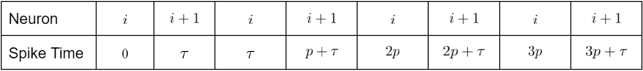
In this case, $w_{i+1,i}$ experiences alternating increases and decreases, with increases having time difference $\tau$ and decreases having time difference $p-\tau.$ Then we have

$\begin{align*} \lim_{t\to\infty} w_{i+1,i}(t) = w_{i+1,i}(0) \lim_{t\to\infty} \left[ \left( 1 + \frac{\alpha}{\exp(k\tau)} \right) \left( 1 - \frac{\alpha}{\exp(k(p-\tau))-\alpha} \right) \right]^{t/p}. \end{align*}$

Thus, the chain solidifies if

$\begin{align*} \left( 1 + \frac{\alpha}{\exp(k\tau)} \right) \left( 1 - \frac{\alpha}{\exp(k(p-\tau))-\alpha} \right) &> 1 \\[5pt] \frac{1}{\exp(k\tau)} - \frac{\alpha + \exp(k\tau)}{\exp(kp)-\alpha\exp(k\tau)} &> 0 \\[5pt] e^{k(p-\tau)}-2\alpha + e^{kt} &> 0. \end{align*}$

Letting $\alpha \to 0,$ we reach $p > 2\tau.$ Thus, if $p>2\tau$, then the chain solidifies, but if $\tau < p \leq 2\tau,$ then the chain breaks.

Case 4. If $\frac{1}{2} \tau < p < \tau$ then the order of (shifted) spike times is as follows:

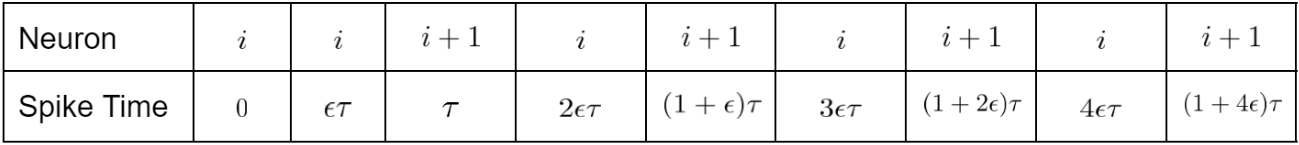
We see that, $w_{i+1,i}$ experiences alternating increases and decreases, with increases having time difference $(1-\epsilon)\tau = \tau-p$, and decreases having time difference $(2\epsilon-1)\tau = 2p-\tau.$ Then we have

$\begin{align*} \lim_{t\to\infty} w_{i+1,i}(t) = w_{i+1,i}(0) \lim_{t\to\infty} \left[ \left( 1 + \frac{\alpha}{\exp(k(\tau-p))} \right) \left( 1 - \frac{\alpha}{\exp(k(2p-\tau))-\alpha} \right) \right]^{t/p}. \end{align*}$

Thus, the chain solidifies if

$\begin{align*} \left( 1 + \frac{\alpha}{\exp(k(\tau-p))} \right) \left( 1 - \frac{\alpha}{\exp(k(2p-\tau))-\alpha} \right) &> 1 \\[5pt] \frac{1}{\exp(k(\tau-p))} - \frac{\alpha + \exp(k(p-\tau)}{\exp(kp)-\alpha\exp(k(p-\tau))} &> 0 \\[5pt] e^{k(2p-\tau)}-\alpha e^{2k(p-\tau)} - \alpha - e^{k(p-t)} &> 0. \end{align*}$

Letting $\alpha \to 0,$ we reach $e^{k(2p-\tau)} > e^{k(p-\tau)},$ which is always true. Thus, the chain solidifies. ■

We are now concerned with breaking or solidifying a particular segment of a tree, since the Proposition gives us a way to break or solidify any subtree as a whole.

Corollary. Suppose that two neurons are stimulated with periods $p$ and $q$, where $q$ is applied to the neuron deeper in the tree. To solidify the connections between $p$ and $q$ while allowing the subtree under $q$ to remain fluid, we can choose

$q=\frac{1}{2}\tau$ and $p=\frac{n}{2}\tau$, where $n>4$, or
$q=\tau$ and $p=n\tau$, where $n>2$.

To break the connections between $p$ and $q$ while allowing the subtree under $q$ to remain fluid, we can choose

$q=\frac{1}{2}\tau$ and $p=\frac{3}{2}\tau$ or $p=2\tau$, or
$q=\tau$ and $p=2\tau$.

Proof. From the Proposition, we see that to solidify the connections between $p$ and $q,$ we must have $\frac{1}{2}\tau < p < \tau$ or $2\tau < p,$ and to break the connections between $p$ and $q,$ we must have $\tau < p \leq 2\tau.$ To ensure that the subtree under $q$ remains fluid, we can choose $q=\frac{1}{2}\tau$ or $q=\tau$ and choose $p$ such that its pulses are canceled by the stimulation at $q.$ ■

Future Directions

One direction for future work is in expanding the theoretical analysis to more initial topologies, such as recombining trees, cycles, unions of cycles, and bidirectional networks. Another direction for future work is in making the model more realistic: one could

include latent weights that can solidify but cannot cause the postsynaptic neuron to spike until solidified, or
run simulations with e.g. leaky integrate-and-fire neurons.

References

[1] Tovee, M. J. (1994). Neuronal Processing: How fast is the speed of thought? Current Biology, 4(12), 1125-1127.

[2] Jesper Sjostrom and Wulfram Gerstner (2010) Spike-timing dependent plasticity. Scholarpedia, 5(2):1362.

Want to get notified about new posts? Join the mailing list and follow on X/Twitter.