Matrix diagonalization can be applied to construct closed-form expressions for recursive sequences.
This post is part of the book Justin Math: Linear Algebra. Suggested citation: Skycak, J. (2019). Recursive Sequence Formulas via Diagonalization. In Justin Math: Linear Algebra. https://justinmath.com/recursive-sequence-formulas-via-diagonalization/
Want to get notified about new posts? Join the mailing list and follow on X/Twitter.
In this chapter, we introduce an interesting application of matrix diagonalization: constructing closed-form expressions for recursive sequences.
Recursive Sequences
A recursive sequence is defined according to one or more initial terms and an update rule for obtaining the next term after some number of previous terms.
For example, the sequences $(a_n)_{n\geq 0}$ and $(b_n)_{n\geq 0}$ given below are arithmetic and geometric sequences given in recursive form.
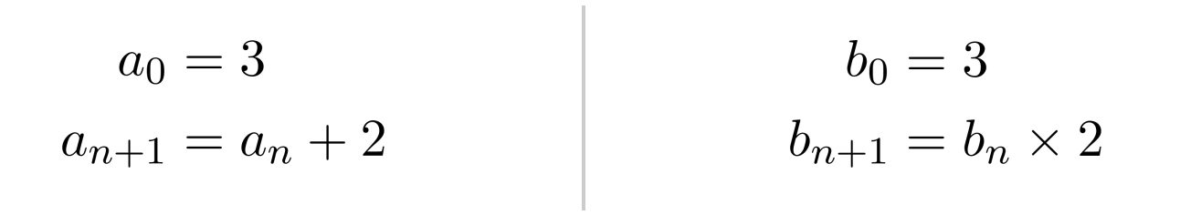
For both of these sequences, it is straightforward to write a closed-form expression for the Nth term:
For other sequences, however, this is not so straightforward. For example, consider the Fibonacci sequence, whose first term is $0$, whose second term is $1$, and whose successive terms are obtained by adding the previous two terms together.
$\begin{align*} 0, 1, 1, 2, 3, 5, 8, 13, 21, 34, \ldots \end{align*}$
The recursive rule for the Fibonacci sequence is as follows:
$\begin{align*} a_0 &= 0 \\ a_1 &= 1 \\ a_{n+2} &= a_n + a_{n+1} \end{align*}$
Finding a Closed-Form Expression
Notice that we can express the recursive update rule using matrices.
$\begin{align*} \begin{pmatrix} a_{n+1} \\ a_{n+2} \end{pmatrix} = \begin{pmatrix} 0 & 1 \\ 1 & 1 \end{pmatrix} \begin{pmatrix} a_n \\ a_{n+1} \end{pmatrix} \end{align*}$
Repeatedly multiplying by this matrix, we can write a closed-form expression for the Nth and (N+1)st terms.
$\begin{align*} \begin{pmatrix} a_{n} \\ a_{n+1} \end{pmatrix} &= \begin{pmatrix} 0 & 1 \\ 1 & 1 \end{pmatrix}^n \begin{pmatrix} a_0 \\ a_{1} \end{pmatrix} \\ &= \begin{pmatrix} 0 & 1 \\ 1 & 1 \end{pmatrix}^n \begin{pmatrix} 0 \\ 1 \end{pmatrix} \end{align*}$
We can simplify this expression even further by diagonalizing the matrix. First, we solve for the eigenvalues.
$\begin{align*} \det \left( \begin{pmatrix}0 & 1 \\ 1 & 1 \end{pmatrix} - \lambda \begin{pmatrix} 1 & 0 \\ 0 & 1 \end{pmatrix} \right) &= 0 \\ \det \begin{pmatrix} -\lambda & 1 \\ 1 & 1-\lambda \end{pmatrix} &= 0 \\ -\lambda(1-\lambda) - (1)(1) &= 0 \\ \lambda^2 - \lambda - 1 &= 0 \\ \lambda &= \frac{1 \pm \sqrt{5}}{2} \end{align*}$
Now, we find the eigenvectors $v_1$ and $v_2$ that correspond to the eigenvalues $\lambda_1 = \frac{1+\sqrt{5} }{2}$ and $\lambda_2 = \frac{1- \sqrt{5} }{2}$.
$\begin{align*} \left( \begin{pmatrix} 0 & 1 \\ 1 & 1 \end{pmatrix} - \left( \frac{1+\sqrt{5}}{2} \right) \begin{pmatrix} 1 & 0 \\ 0 & 1 \end{pmatrix} \right) v_1 &= \begin{pmatrix} 0 \\ 0 \end{pmatrix} \\ \begin{pmatrix} -\frac{1+\sqrt{5}}{2} & 1 \\ 1 & \frac{1-\sqrt{5}}{2} \end{pmatrix} v_1 &= \begin{pmatrix} 0 \\ 0 \end{pmatrix} \\ \begin{pmatrix} 2 & 0 \\ 0 & \frac{1+\sqrt{5}}{2} \end{pmatrix} \begin{pmatrix} -\frac{1+\sqrt{5}}{2} & 1 \\ 1 & \frac{1-\sqrt{5}}{2} \end{pmatrix} v_1 &= \begin{pmatrix} 2 & 0 \\ 0 & \frac{1+\sqrt{5}}{2} \end{pmatrix} \begin{pmatrix} 0 \\ 0 \end{pmatrix} \\ \begin{pmatrix}1+\sqrt{5} & -2 \\ 1+\sqrt{5} & -2 \end{pmatrix} v_1 &= \begin{pmatrix} 0 \\ 0 \end{pmatrix} \\ v_1 &= \begin{pmatrix} 2 \\ 1+\sqrt{5} \end{pmatrix} \end{align*}$
$\begin{align*} \left( \begin{pmatrix} 0 & 1 \\ 1 & 1 \end{pmatrix} - \left( \frac{1-\sqrt{5}}{2} \right) \begin{pmatrix} 1 & 0 \\ 0 & 1 \end{pmatrix} \right) v_2 &= \begin{pmatrix} 0 \\ 0 \end{pmatrix} \\ \begin{pmatrix} \frac{-1+\sqrt{5}}{2} & 1 \\ 1 & \frac{1+\sqrt{5}}{2} \end{pmatrix} v_2 &= \begin{pmatrix} 0 \\ 0 \end{pmatrix} \\ \begin{pmatrix} 2 & 0 \\ 0 & \frac{1-\sqrt{5}}{2} \end{pmatrix} \begin{pmatrix} \frac{-1+\sqrt{5}}{2} & 1 \\ 1 & \frac{1+\sqrt{5}}{2} \end{pmatrix} v_2 &= \begin{pmatrix} 2 & 0 \\ 0 & \frac{1-\sqrt{5}}{2} \end{pmatrix} \begin{pmatrix} 0 \\ 0 \end{pmatrix} \\ \begin{pmatrix}-1+\sqrt{5} & 2 \\ -1+\sqrt{5} & 2 \end{pmatrix} v_2 &= \begin{pmatrix} 0 \\ 0 \end{pmatrix} \\ v_2 &= \begin{pmatrix} 2 \\ 1-\sqrt{5} \end{pmatrix} \end{align*}$
Finally, we can diagonalize the matrix.
$\begin{align*} \begin{pmatrix} 0 & 1 \\ 1 & 1 \end{pmatrix} &= \begin{pmatrix} 2 & 2 \\ 1+\sqrt{5} & 1-\sqrt{5} \end{pmatrix} \begin{pmatrix} \frac{1+\sqrt{5}}{2} & 0 \\ 0 & \frac{1-\sqrt{5}}{2} \end{pmatrix} \begin{pmatrix} 2 & 2 \\ 1+\sqrt{5} & 1-\sqrt{5} \end{pmatrix}^{-1} \end{align*}$
Substituting the diagonalized matrix into the original formula, we are able to simplify so much that we find a closed-form, non-matrix formula for the Nth term of the sequence.
$\begin{align*} \begin{pmatrix} a_{n} \\ a_{n+1} \end{pmatrix} &= \begin{pmatrix} 0 & 1 \\ 1 & 1 \end{pmatrix}^n \begin{pmatrix} 0 \\ 1 \end{pmatrix} \\ \begin{pmatrix} a_n \\ a_{n+1} \end{pmatrix} &= \left[ \begin{pmatrix} 2 & 2 \\ 1+\sqrt{5} & 1-\sqrt{5} \end{pmatrix} \begin{pmatrix} \frac{1+\sqrt{5}}{2} & 0 \\ 0 & \frac{1-\sqrt{5}}{2} \end{pmatrix} \begin{pmatrix} 2 & 2 \\ 1+\sqrt{5} & 1-\sqrt{5} \end{pmatrix}^{-1} \right]^n \begin{pmatrix} 0 \\ 1 \end{pmatrix} \\ \begin{pmatrix} a_n \\ a_{n+1} \end{pmatrix} &= \begin{pmatrix} 2 & 2 \\ 1+\sqrt{5} & 1-\sqrt{5} \end{pmatrix} \begin{pmatrix} \left( \frac{1+\sqrt{5}}{2} \right)^n & 0 \\ 0 & \left( \frac{1-\sqrt{5}}{2} \right)^n \end{pmatrix} \begin{pmatrix} 2 & 2 \\ 1+\sqrt{5} & 1-\sqrt{5} \end{pmatrix}^{-1}\begin{pmatrix} 0 \\ 1 \end{pmatrix} \\ \begin{pmatrix} a_n \\ a_{n+1} \end{pmatrix} &= \begin{pmatrix} 2 & 2 \\ 1+\sqrt{5} & 1-\sqrt{5} \end{pmatrix} \begin{pmatrix} \left( \frac{1+\sqrt{5}}{2} \right)^n & 0 \\ 0 & \left( \frac{1-\sqrt{5}}{2} \right)^n \end{pmatrix} \left[ \frac{1}{-4\sqrt{5}} \begin{pmatrix} 1-\sqrt{5} & -2 \\ -1-\sqrt{5} & 2 \end{pmatrix} \right] \begin{pmatrix} 0 \\ 1 \end{pmatrix} \\ \begin{pmatrix} a_n \\ a_{n+1} \end{pmatrix} &= \frac{1}{2\sqrt{5}} \begin{pmatrix} 2 & 2 \\ 1+\sqrt{5} & 1-\sqrt{5} \end{pmatrix} \begin{pmatrix} \left( \frac{1+\sqrt{5}}{2} \right)^n & 0 \\ 0 & \left( \frac{1-\sqrt{5}}{2} \right)^n \end{pmatrix} \begin{pmatrix} 1 \\ -1 \end{pmatrix} \\ \begin{pmatrix} a_n \\ a_{n+1} \end{pmatrix} &= \frac{1}{\sqrt{5}} \begin{pmatrix} 1 & 1 \\ \frac{1+\sqrt{5}}{2} & \frac{1-\sqrt{5}}{2} \end{pmatrix} \begin{pmatrix} \left( \frac{1+\sqrt{5}}{2} \right)^n \\ - \left( \frac{1-\sqrt{5}}{2} \right)^n \end{pmatrix} \\ \begin{pmatrix} a_n \\ a_{n+1} \end{pmatrix} &= \begin{pmatrix} \frac{1}{\sqrt{5}} \left[ \left( \frac{1+\sqrt{5}}{2} \right)^n - \left( \frac{1-\sqrt{5}}{2} \right)^n \right] \\ \frac{1}{\sqrt{5}} \left[ \left( \frac{1+\sqrt{5}}{2} \right)^{n+1} - \left( \frac{1-\sqrt{5}}{2} \right)^{n+1} \right] \end{pmatrix} \\ a_n &= \frac{1}{\sqrt{5}} \left[ \left( \frac{1+\sqrt{5}}{2} \right)^n - \left( \frac{1-\sqrt{5}}{2} \right)^n \right] \end{align*}$
This formula might be a little surprising – the Fibonacci sequence consists only of whole numbers, yet $\sqrt{5}$ appears often in the formula!
However, the formula is indeed correct. We verify the formula for $a_0$, $a_1$, and $a_2$ – and it will work on all the other terms as well.
$\begin{align*} a_0 &= \frac{1}{\sqrt{5}} \left[ \left( \frac{1+\sqrt{5}}{2} \right)^0 - \left( \frac{1-\sqrt{5}}{2} \right)^0 \right] \\ &= \frac{1}{\sqrt{5}} \left[ 1-1 \right] \\ &= 0 \end{align*}$
$\begin{align*} a_1 &= \frac{1}{\sqrt{5}} \left[ \left( \frac{1+\sqrt{5}}{2} \right)^1 - \left( \frac{1-\sqrt{5}}{2} \right)^1 \right] \\ &= \frac{1}{\sqrt{5}} \left[ \sqrt{5} \right] \\ &= 1 \end{align*}$
$\begin{align*} a_2 &= \frac{1}{\sqrt{5}} \left[ \left( \frac{1+\sqrt{5}}{2} \right)^2 - \left( \frac{1-\sqrt{5}}{2} \right)^2 \right] \\ &= \frac{1}{\sqrt{5}} \left[ \frac{1+2\sqrt{5}+5}{4} - \frac{1-2\sqrt{5}+5}{4} \right] \\ &= \frac{1}{\sqrt{5}} \left[ \sqrt{5} \right] \\ &= 1 \end{align*}$
Case when Approximation is Required
This same method applies for any recursive sequence, though we may need to diagonalize a higher-dimensional matrix and numerically approximate the eigenvalues.
For example, consider the following spin-off of the Fibonacci sequence:
$\begin{align*} a_0 &= 0 \\ a_1 &= 1 \\ a_2 &= 1 \\ a_{n+3} &= 2a_n + a_{n+2} \end{align*}$
First, we express the recursive update rule using matrices, and write a closed-form expression involving an exponentiated matrix multiplying the first few terms.
$\begin{align*} \begin{pmatrix} a_{n+1} \\ a_{n+2} \\ a_{n+3} \end{pmatrix} &= \begin{pmatrix} 0 & 1 & 0 \\ 0 & 0 & 1 \\ 2 & 0 & 1 \end{pmatrix} \begin{pmatrix} a_n \\ a_{n+1} \\ a_{n+2} \end{pmatrix} \\ &= \begin{pmatrix} 0 & 1 & 0 \\ 0 & 0 & 1 \\ 2 & 0 & 1 \end{pmatrix}^n \begin{pmatrix} a_0 \\ a_1 \\ a_2 \end{pmatrix} \\ &= \begin{pmatrix} 0 & 1 & 0 \\ 0 & 0 & 1 \\ 2 & 0 & 1 \end{pmatrix}^n \begin{pmatrix} 0 \\ 1 \\ 1 \end{pmatrix} \end{align*}$
We omit the steps of diagonalizing the matrix since they should be routine by now – but it is worthwhile to discuss the method of approximating the eigenvalues.
When solving for the eigenvalues, we reach the following equation:
$\begin{align*} \lambda^3 - \lambda^2 - 2 = 0 \end{align*}$
This cubic cannot be factored manually – not even using synthetic division – since it has no rational roots.
Hence, we turn to a graphing utility to approximate a root $\lambda_1 \approx 1.696$. Then, we can perform synthetic division with that root to factor the polynomial into
$\begin{align*} (\lambda - 1.696)(\lambda^2 + 0.696 \lambda + 1.180) = 0. \end{align*}$
We can use the quadratic equation to solve
$\begin{align*} \lambda^2 + 0.696\lambda + 1.180 = 0 \end{align*}$
for the other two roots, which we find as $\lambda_2 \approx -0.348-1.029i$ and $\lambda_3 \approx -0.348+1.029i$.
Then, with a bit of grunt work, we can use these approximations to solve for the eigenvectors, substitute the diagonalization into the original equation, and multiply to find the formula for the Nth term.
The result, with each term rounded to 3 decimal places, is
$\begin{align*} a_n \approx \hspace{.1cm} &(-0.162+0.164i)(-0.348-1.029i)^n \\ &- (0.162+0.164i)(-0.348+1.029i)^n \\ &+ 0.324(1.696)^n \, . \end{align*}$
Lastly, we can verify that the first several terms match up with the actual sequence $0, 1, 1, 1, 3, 5, 7, 13$.
Our estimates are slightly off due to compounded rounding error, but they could be made more accurate by using greater precision in the decimals that occur in the formula for $a_n$.
$\begin{align*} \begin{matrix} a_0 = 0 & a_1 \approx 1.000 & a_2 \approx 1.001 & a_3 \approx 1.001 \\ a_4 \approx 3.003 & a_5 \approx 5.006 & a_6 \approx 7.011 & a_7 \approx 13.022 \end{matrix} \end{align*}$
Exercises
Use diagonalization to compute a closed-form expression for the recursive sequence $a_n$. (You can view the solution by clicking on the problem.)
$\begin{align*} 1) \hspace{.75cm} a_0 &= 0 \\ a_1 &= 1 \\ a_{n+2} &= 2a_n + a_{n+1} \end{align*}$
Solution:
$\begin{align*} a_n = \frac{2^n-(-1)^n}{3} \end{align*}$
$\begin{align*} 2) \hspace{.75cm} a_0 &= 0 \\ a_1 &= 1 \\ a_{n+2} &= a_n + 2a_{n+1} \end{align*}$
Solution:
$\begin{align*} a_n = \frac{1}{2\sqrt{2}} \left[ \left( 1+\sqrt{2} \right)^n - \left( 1-\sqrt{2} \right)^n \right] \end{align*}$
$\begin{align*} 3) \hspace{.75cm} a_0 &= 0 \\ a_1 &= 1 \\ a_2 &= 1 \\ a_{n+3} &= a_n + a_{n+2} \end{align*}$
Solution:
$\begin{align*} a_n \approx \hspace{.1cm} &(-0.209+0.184i)(-0.233-0.793i)^n \\ &- (0.209+0.184i)(-0.233+0.793i)^n \\ &+ 0.417(1.466)^n \end{align*}$
$\begin{align*} 4) \hspace{.75cm} a_0 &= 0 \\ a_1 &= 1 \\ a_2 &= 1 \\ a_{n+3} &= a_n + a_{n+1}+ a_{n+2} \end{align*}$
Solution:
$\begin{align*} a_n \approx \hspace{.1cm} &(-0.168+0.198i)(-0.420-0.606i)^n \\ &- (0.168+0.198i)(-0.420+0.606i)^n \\ &+ 0.336(1.839)^n \end{align*}$
This post is part of the book Justin Math: Linear Algebra. Suggested citation: Skycak, J. (2019). Recursive Sequence Formulas via Diagonalization. In Justin Math: Linear Algebra. https://justinmath.com/recursive-sequence-formulas-via-diagonalization/
Want to get notified about new posts? Join the mailing list and follow on X/Twitter.