Linear Systems as Transformations of Vectors by Matrices

by Justin Skycak (@justinskycak) on August 01, 2019

Matrices are vectors whose components are themselves vectors.

This post is part of the book Justin Math: Linear Algebra. Suggested citation: Skycak, J. (2019). Linear Systems as Transformations of Vectors by Matrices. In Justin Math: Linear Algebra. https://justinmath.com/linear-systems-as-transformations-of-vectors-by-matrices/

Want to get notified about new posts? Join the mailing list and follow on X/Twitter.

Let’s create a compact notation for expressing systems of linear equations like the one shown below.

Matrices of Column Vectors

We’re familiar with a slightly condensed version using coefficient vectors.

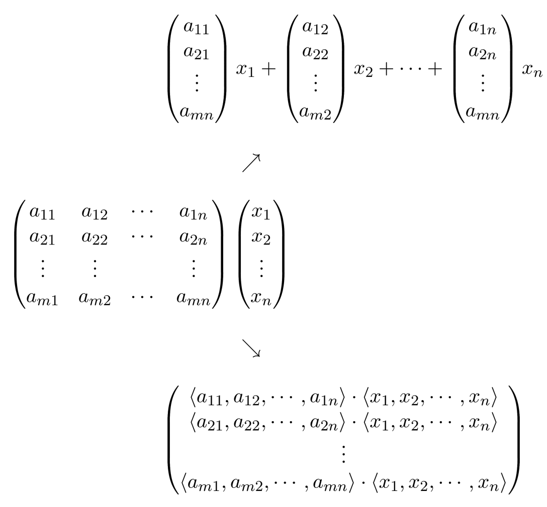
$\begin{align*} \begin{pmatrix} a_{11} \\ a_{21} \\ \vdots \\ a_{mn} \end{pmatrix} x_1 + \begin{pmatrix} a_{12} \\ a_{22} \\ \vdots \\ a_{m2} \end{pmatrix} x_2 + \cdots + \begin{pmatrix} a_{1n} \\ a_{2n} \\ \vdots \\ a_{mn} \end{pmatrix} x_n = \begin{pmatrix} b_1 \\ b_2 \\ \vdots \\ b_m \end{pmatrix} \end{align*}$

However, we can condense this even further by putting the coefficient vectors in a vector themselves and taking the dot product with the vector of variables.

$\begin{align*} \begin{pmatrix} \begin{pmatrix} a_{11} \\ a_{21} \\ \vdots \\ a_{mn} \end{pmatrix}, \begin{pmatrix} a_{12} \\ a_{22} \\ \vdots \\ a_{m2} \end{pmatrix}, \cdots, \begin{pmatrix} a_{1n} \\ a_{2n} \\ \vdots \\ a_{mn} \end{pmatrix} \end{pmatrix} \cdot \left< x_1, x_2, \cdots, x_n \right> = \begin{pmatrix} b_1 \\ b_2 \\ \vdots \\ b_m \end{pmatrix} \end{align*}$

To save space, the vector of variables can be written as a column vector as well.

$\begin{align*} \begin{pmatrix} \begin{pmatrix} a_{11} \\ a_{21} \\ \vdots \\ a_{mn} \end{pmatrix}, \begin{pmatrix} a_{12} \\ a_{22} \\ \vdots \\ a_{m2} \end{pmatrix}, \cdots, \begin{pmatrix} a_{1n} \\ a_{2n} \\ \vdots \\ a_{mn} \end{pmatrix} \end{pmatrix} \cdot \begin{pmatrix} x_1 \\ x_2 \\ \vdots \\ x_n \end{pmatrix} = \begin{pmatrix} b_1 \\ b_2 \\ \vdots \\ b_m \end{pmatrix} \end{align*}$

Finally, to simplify the notation, we can remove the vector braces around the individual coefficient vectors and remove the dot product symbol.

The array containing the coefficients is called a matrix. It’s really just a vector of sub-vectors, written without braces on the individual sub-vectors.

Looking back, it makes sense to define a matrix multiplying a vector as follows:

$\begin{align*} \begin{pmatrix} a_{11} & a_{12} & \cdots & a_{1n} \\ a_{21} & a_{22} & \cdots & a_{2n} \\ \vdots & \vdots & & \vdots \\ a_{m1} & a_{m2} & \cdots & a_{mn} \end{pmatrix} \begin{pmatrix} x_1 \\ x_2 \\ \vdots \\ x_n \end{pmatrix} \rightarrow \begin{pmatrix} a_{11} \\ a_{21} \\ \vdots \\ a_{mn} \end{pmatrix} x_1 + \begin{pmatrix} a_{12} \\ a_{22} \\ \vdots \\ a_{m2} \end{pmatrix} x_2 + \cdots + \begin{pmatrix} a_{1n} \\ a_{2n} \\ \vdots \\ a_{mn} \end{pmatrix} x_n \end{align*}$

Matrices of Row Vectors

Keeping this form of matrix notation and multiplication in mind, let’s start from scratch and proceed to condense a system of linear equations in a different way. We’ll get an interesting result.

Again, we will start with the system below.

This time, however, we will begin by writing each equation as a dot product.

$\begin{align*} \left< a_{11}, a_{12}, \cdots, a_{1n} \right> \cdot \left< x_1, x_2, \cdots, x_n \right> &= b_1 \\ \left< a_{21}, a_{22}, \cdots, a_{2n} \right> \cdot \left< x_1, x_2, \cdots, x_n \right> &= b_2 \\ &\vdots \\ \left< a_{m1}, a_{m2}, \cdots, a_{mn} \right> \cdot \left< x_1, x_2, \cdots, x_n \right> &= b_m \end{align*}$

Then, we will write the system as a single vector equation by interpreting each side of the equation as a vector.

$\begin{align*} \begin{pmatrix} \left< a_{11}, a_{12}, \cdots, a_{1n} \right> \cdot \left< x_1, x_2, \cdots, x_n \right> \\ \left< a_{21}, a_{22}, \cdots, a_{2n} \right> \cdot \left< x_1, x_2, \cdots, x_n \right> \\ \vdots \\ \left< a_{m1}, a_{m2}, \cdots, a_{mn} \right> \cdot \left< x_1, x_2, \cdots, x_n \right> \end{pmatrix} = \begin{pmatrix} b_1 \\ b_2 \\ \vdots \\ b_m \end{pmatrix} \end{align*}$

Each component of the left-hand-side vector includes a dot product with the vector of variables, so we can factor out the vector of variables.

$\begin{align*} \begin{pmatrix} \left< a_{11}, a_{12}, \cdots, a_{1n} \right> \\ \left< a_{21}, a_{22}, \cdots, a_{2n} \right> \\ \vdots \\ \left< a_{m1}, a_{m2}, \cdots, a_{mn} \right> \end{pmatrix} \left< x_1, x_2, \cdots, x_n \right> = \begin{pmatrix} b_1 \\ b_2 \\ \vdots \\ b_m \end{pmatrix} \end{align*}$

Again, to save space, the vector of variables can be written as a column vector.

$\begin{align*} \begin{pmatrix} \left< a_{11}, a_{12}, \cdots, a_{1n} \right> \\ \left< a_{21}, a_{22}, \cdots, a_{2n} \right> \\ \vdots \\ \left< a_{m1}, a_{m2}, \cdots, a_{mn} \right> \end{pmatrix} \begin{pmatrix} x_1 \\ x_2 \\ \vdots \\ x_n \end{pmatrix} = \begin{pmatrix} b_1 \\ b_2 \\ \vdots \\ b_m \end{pmatrix} \end{align*}$

Finally, to simplify the notation, we can again remove the vector braces around the individual coefficient vectors.

Again, there is a matrix! And again, the matrix just represents a vector of sub-vectors, written without braces on the individual sub-vectors.

But this time, looking back, it makes sense to define a matrix multiplying a vector by a different rule.

$\begin{align*} \begin{pmatrix} a_{11} & a_{12} & \cdots & a_{1n} \\ a_{21} & a_{22} & \cdots & a_{2n} \\ \vdots & \vdots & & \vdots \\ a_{m1} & a_{m2} & \cdots & a_{mn} \end{pmatrix} \begin{pmatrix} x_1 \\ x_2 \\ \vdots \\ x_n \end{pmatrix} \rightarrow \begin{pmatrix} \left< a_{11}, a_{12}, \cdots, a_{1n} \right> \cdot \left< x_1, x_2, \cdots, x_n \right> \\ \left< a_{21}, a_{22}, \cdots, a_{2n} \right> \cdot \left< x_1, x_2, \cdots, x_n \right> \\ \vdots \\ \left< a_{m1}, a_{m2}, \cdots, a_{mn} \right> \cdot \left< x_1, x_2, \cdots, x_n \right> \end{pmatrix} \end{align*}$

Matrix Multiplication

Which rule is correct? It turns out, they both are. Before we do an example, though, let’s recap.

We’re stumbling upon the following structure:

$\begin{align*} \begin{matrix} a_{11}x_1 &+& a_{12}x_2 &+& \cdots &+& a_{1n}x_n &=& b_1 \\ a_{21}x_1 &+& a_{22}x_2 &+& \cdots &+& a_{2n}x_n &=& b_2 \\ & & & & & & &\vdots& \\ a_{m1}x_1 &+& a_{m2}x_2 &+& \cdots &+& a_{mn}x_n &=& b_m \end{matrix}& \\ \text{ } \\ \begin{pmatrix} a_{11} & a_{12} & \cdots & a_{1n} \\ a_{21} & a_{22} & \cdots & a_{2n} \\ \vdots & \vdots & & \vdots \\ a_{m1} & a_{m2} & \cdots & a_{mn} \end{pmatrix} \begin{pmatrix} x_1 \\ x_2 \\ \vdots \\ x_n \end{pmatrix} = \begin{pmatrix} b_1 \\ b_2 \\ \vdots \\ b_m \end{pmatrix}& \end{align*}$

The array on the left-hand side is called a matrix, and we have two ways to compute the product of a matrix and a vector – one which involves interpreting the columns of the matrix as individual vectors, and another which involves interpreting the rows of the matrix as individual vectors.

To verify that both methods of computation indeed yield the same result, we can try out a simple example using the two different methods to compute the product of a 2-by-2 matrix and a 2-dimensional vector.

$\begin{align*} &\begin{pmatrix} 1 & 2 \\ 3 & 4 \end{pmatrix} \begin{pmatrix} 5 \\ 6 \end{pmatrix} = \begin{pmatrix} 1 \\ 3 \end{pmatrix} (5) + \begin{pmatrix} 2 \\ 4 \end{pmatrix} (6) = \begin{pmatrix} 5 \\ 15 \end{pmatrix} + \begin{pmatrix} 12 \\ 24 \end{pmatrix} = \begin{pmatrix} 17 \\ 39 \end{pmatrix} \\ \text{ } \\ &\begin{pmatrix} 1 & 2 \\ 3 & 4 \end{pmatrix} \begin{pmatrix} 5 \\ 6 \end{pmatrix} = \begin{pmatrix} \left< 1, 2 \right> \cdot \left< 5,6 \right> \\ \left< 3, 4 \right> \cdot \left< 5,6 \right> \end{pmatrix} = \begin{pmatrix} 5 + 12 \\ 15 + 24 \end{pmatrix} = \begin{pmatrix} 17 \\ 39 \end{pmatrix} \end{align*}$

Geometric Intuition

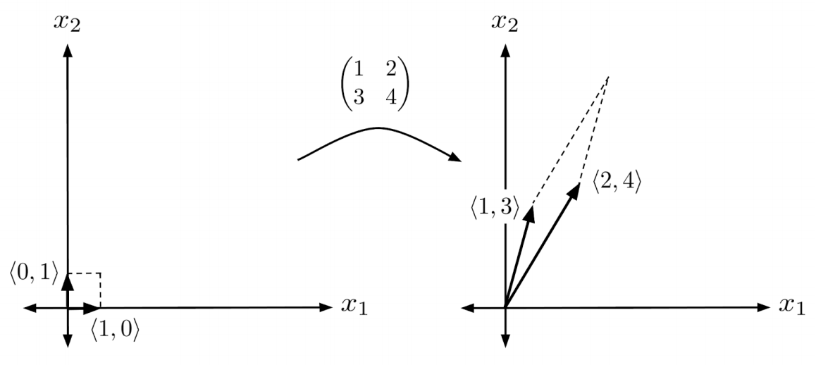
Lastly, let’s build some geometric intuition. Geometrically, a matrix represents a transformation of a vector space, and we can visualize this transformation by thinking about what the matrix does to the N-dimensional unit cube.

For example, to see what the matrix from the example does to the unit square, we can multiply the vertices $(1,0)$ and $(0,1)$ of the unit square by the matrix.

$\begin{align*} &\begin{pmatrix} 1 & 2 \\ 3 & 4 \end{pmatrix} \begin{pmatrix} 1 \\ 0 \end{pmatrix} = \begin{pmatrix} 1 \\ 3 \end{pmatrix} (1) + \begin{pmatrix} 2 \\ 4 \end{pmatrix} (0) = \begin{pmatrix} 1 \\ 3 \end{pmatrix} \\ \text{ } \\ &\begin{pmatrix} 1 & 2 \\ 3 & 4 \end{pmatrix} \begin{pmatrix} 0 \\ 1 \end{pmatrix}= \begin{pmatrix} 1 \\ 3 \end{pmatrix} (0) + \begin{pmatrix} 2 \\ 4 \end{pmatrix} (1) = \begin{pmatrix} 2 \\ 4 \end{pmatrix} \end{align*}$

We see that the matrix moves the vertices of the unit square from $(1,0)$ and $(0,1)$, to $(1,2)$ and $(3,4)$. Notice that these are just the columns of the matrix!

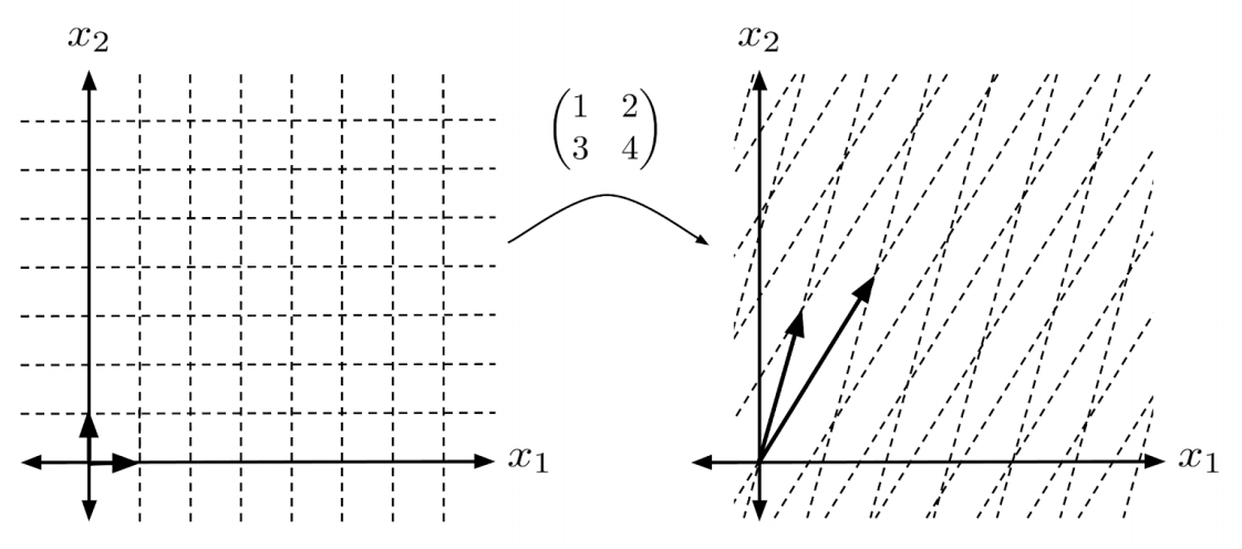
But it’s not just the unit square that is transformed in this way. The entire space undergoes this transformation as well.

And it’s more than simple stretching – the space is actually flipped over, since the original bottom vertex $(1,0)$ is now the top vertex $(1,3)$, and the original top vertex $(0,1)$ is now the bottom vertex $(2,4)$.

Exercises

Convert the following linear systems to matrix form. (You can view the solution by clicking on the problem.)

$\begin{align*} 1) \hspace{.5cm} 3x_1 -2x_2 &= 7 \\ 5x_1 + 4x_2 &= 6 \end{align*}$

Solution:
$\begin{align*} \begin{pmatrix} 3 & -2 \\ 5 & 4 \end{pmatrix} \begin{pmatrix} x_1 \\ x_2 \end{pmatrix} = \begin{pmatrix} 7 \\ 6 \end{pmatrix} \end{align*}$

$\begin{align*} 2) \hspace{.5cm} x_1 - 8x_2 &= 3 \\ x_1+x_2&=-2 \end{align*}$

Solution:
$\begin{align*} \begin{pmatrix}1 & -8 \\ 1 & 1 \end{pmatrix} \begin{pmatrix} x_1 \\ x_2 \end{pmatrix} = \begin{pmatrix} 3 \\ -2 \end{pmatrix} \end{align*}$

$\begin{align*} 3) \hspace{.5cm} 2x_1+3x_2&=4 \\ 5x_1 &= 8 \end{align*}$

Solution:
$\begin{align*} \begin{pmatrix} 2 & 3 \\ 5 & 0 \end{pmatrix} \begin{pmatrix} x_1 \\ x_2 \end{pmatrix} = \begin{pmatrix} 4 \\ 8 \end{pmatrix} \end{align*}$

$\begin{align*} 4) \hspace{.5cm} \hspace{1cm} 8x_2 &= -7 \\ 3x_1 - x_2 &= 5 \end{align*}$

Solution:
$\begin{align*} \begin{pmatrix} 0 & 8 \\ 3 & -1 \end{pmatrix} \begin{pmatrix} x_1 \\ x_2 \end{pmatrix} = \begin{pmatrix} -7 \\ 5 \end{pmatrix} \end{align*}$

$\begin{align*} 5) \hspace{.5cm} 2x_1+3x_2-4x_3 &= 5 \\ 7x_1 - 2x_2 + 3x_3 &= 2 \\ 9x_2 + 5x_2 + 4x_3 &= 1 \end{align*}$

Solution:
$\begin{align*} \begin{pmatrix} 2 & 3 & -4 \\ 7 & -2 & 3 \\ 9 & 5 & 4 \end{pmatrix} \begin{pmatrix} x_1 \\ x_2 \\ x_3\end{pmatrix} = \begin{pmatrix} 5 \\ 2 \\ 1 \end{pmatrix} \end{align*}$

$\begin{align*} 6) \hspace{.5cm} \hspace{.5cm}x_1 - x_2 + x_3 &= 0 \\ 2x_1 - 5x_2 + x_3 &= -2 \\ x_1 + 4x_2 + 2x_3 &= 3 \end{align*}$

Solution:
$\begin{align*} \begin{pmatrix}1 & -1 & 1 \\ 2 & -5 & 1 \\ 1 & 4 & 2 \end{pmatrix} \begin{pmatrix} x_1 \\ x_2 \\ x_3\end{pmatrix} = \begin{pmatrix} 0 \\ -2 \\ 3 \end{pmatrix} \end{align*}$

$\begin{align*} 7) \hspace{.5cm} \hspace{1cm} x_1-x_3 &= 4 \\ x_2 + 3x_3 &= 7 \\ x_1 + x_2 + x_3 &= -5 \end{align*}$

Solution:
$\begin{align*} \begin{pmatrix} 1 & 0 & -1 \\ 0 & 1 & 3 \\ 1 & 1 & 1 \end{pmatrix} \begin{pmatrix} x_1 \\ x_2 \\ x_3\end{pmatrix} = \begin{pmatrix} 4 \\ 7 \\ -5 \end{pmatrix} \end{align*}$

$\begin{align*} 8) \hspace{.5cm} x_2 + x_3 &= 6 \\ x_1 + x_3 &= 5 \\ x_1 + x_2 &= 4 \end{align*}$

Solution:
$\begin{align*} \begin{pmatrix} 0 & 1 & 1 \\ 1 & 0 & 1 \\ 1 & 1 & 0 \end{pmatrix} \begin{pmatrix} x_1 \\ x_2 \\ x_3\end{pmatrix} = \begin{pmatrix} 6 \\ 5 \\ 4 \end{pmatrix} \end{align*}$

$\begin{align*} 9) \hspace{.5cm} x_1+x_2+x_3-x_4 &= 7 \\ x_2+x_3-7x_4 &= 5 \\ x_1 +8x_3 &= 11 \\ 4x_2+x_4 &= 3 \end{align*}$

Solution:
$\begin{align*} \begin{pmatrix} 1 & 1 & 1 & -1 \\ 0 & 1 & 1 & -7 \\ 1 & 0 & 8 & 0 \\ 0 & 4 & 0 & 1 \end{pmatrix} \begin{pmatrix} x_1 \\ x_2 \\ x_3 \\ x_4 \end{pmatrix} = \begin{pmatrix} 7 \\ 5 \\ 11 \\ 3 \end{pmatrix} \end{align*}$

$\begin{align*} 10) \hspace{.5cm} x_1-2x_2+3x_3 &= 0 \\ x_2-2x_3+3x_4 &= 0 \\ x_1 - 2x_3 + 3x_4 &= 1 \\ x_1 - 2x_2 + 3x_4 &= 1 \end{align*}$

Solution:
$\begin{align*} \begin{pmatrix} 1 & -2 & 3 & 0 \\ 0 & 1 & -2 & 3 \\ 1 & 0 & -2 & 3 \\ 1 & -2 & 0 & 3 \end{pmatrix} \begin{pmatrix} x_1 \\ x_2 \\ x_3 \\ x_4 \end{pmatrix} = \begin{pmatrix} 0 \\ 0 \\ 1 \\ 1 \end{pmatrix} \end{align*}$

Compute the product of the given vector and matrix by A) interpreting the columns of the matrix as individual vectors, and B) interpreting the rows of the matrix as individual vectors. Verify that the results are the same. (You can view the solution by clicking on the problem.)

$\begin{align*} 11) \hspace{.5cm} \begin{pmatrix} 1 & 3 \\ 4 & 1 \end{pmatrix} \begin{pmatrix} 2 \\ 5 \end{pmatrix} \end{align*}$

Solution:
$\begin{align*} \begin{pmatrix} 17 \\ 13 \end{pmatrix} \end{align*}$

$\begin{align*} 12) \hspace{.5cm} \begin{pmatrix} -2 & 1 \\ 3 & 1 \end{pmatrix} \begin{pmatrix} -1 \\ 2 \end{pmatrix} \end{align*}$

Solution:
$\begin{align*} \begin{pmatrix}4 \\ -1 \end{pmatrix} \end{align*}$

$\begin{align*} 13) \hspace{.5cm} \begin{pmatrix} 7 & 2 \\ 1 & 4 \end{pmatrix} \begin{pmatrix} -3 \\ 1 \end{pmatrix} \end{align*}$

Solution:
$\begin{align*} \begin{pmatrix} -19 \\ 1 \end{pmatrix} \end{align*}$

$\begin{align*} 14) \hspace{.5cm} \begin{pmatrix} 3 & 0 \\ 2 & -3 \end{pmatrix} \begin{pmatrix} 0 \\ 4 \end{pmatrix} \end{align*}$

Solution:
$\begin{align*} \begin{pmatrix} 0 \\ -12 \end{pmatrix} \end{align*}$

$\begin{align*} 15) \hspace{.5cm} \begin{pmatrix} 1 & 3 & 2 \\ -1 & 0 & 1 \\ 2 & 1 & 0 \end{pmatrix} \begin{pmatrix} 2 \\ 1 \\ 3 \end{pmatrix} \end{align*}$

Solution:
$\begin{align*} \begin{pmatrix} 11 \\ 1 \\ 5 \end{pmatrix} \end{align*}$

$\begin{align*} 16) \hspace{.5cm} \begin{pmatrix} 3 & 1 & 0 \\ 2 & 0 & 1 \\ -1 & 2 & -3 \end{pmatrix} \begin{pmatrix} 5 \\ 1 \\ 0 \end{pmatrix} \end{align*}$

Solution:
$\begin{align*} \begin{pmatrix} 16 \\ 10 \\ -3 \end{pmatrix} \end{align*}$

$\begin{align*} 17) \hspace{.5cm} \begin{pmatrix} 1 & 2 & 0 \\ 4 & 3 & 1 \\ 3 & -1 & -1 \end{pmatrix} \begin{pmatrix} -1 \\ 1 \\ 2 \end{pmatrix} \end{align*}$

Solution:
$\begin{align*} \begin{pmatrix} 1 \\ -3 \\ -2 \end{pmatrix} \end{align*}$

$\begin{align*} 18) \hspace{.5cm} \begin{pmatrix} 2 & 3 & 0 \\ 5 & 0 & 1 \\ 1 & 1 & 2 \end{pmatrix} \begin{pmatrix} 5 \\ -2 \\ 3 \end{pmatrix} \end{align*}$

Solution:
$\begin{align*} \begin{pmatrix} 4 \\ 28 \\ 9 \end{pmatrix} \end{align*}$

$\begin{align*} 19) \hspace{.5cm} \begin{pmatrix} 1 & 3 & 2 & 1 \\ 0 & 0 & 3 & 4 \\ 1 & 0 & -1 & -2 \\ 3 & -4 & -2 & 1 \end{pmatrix} \begin{pmatrix} 1 \\ 3 \\ 2 \\ 0 \end{pmatrix} \end{align*}$

Solution:
$\begin{align*} \begin{pmatrix} 14 \\ 6 \\ -1 \\ -13 \end{pmatrix} \end{align*}$

$\begin{align*} 20) \hspace{.5cm} \begin{pmatrix} 7 & 0 & -1 & -1 \\ 2 & 3 & -1 & -2 \\ 0 & 1 & 2 & 3 \\ 4 & 3 & -2 & 1 \end{pmatrix} \begin{pmatrix} 3 \\ 1 \\ -1 \\ 2 \end{pmatrix} \end{align*}$

Solution:
$\begin{align*} \begin{pmatrix} 20 \\ 6 \\ 5 \\ 19 \end{pmatrix} \end{align*}$

Want to get notified about new posts? Join the mailing list and follow on X/Twitter.