K-Nearest Neighbors

by Justin Skycak (@justinskycak) on January 07, 2022

One of the simplest classifiers.

This post is part of the book Introduction to Algorithms and Machine Learning: from Sorting to Strategic Agents. Suggested citation: Skycak, J. (2022). K-Nearest Neighbors. In Introduction to Algorithms and Machine Learning: from Sorting to Strategic Agents. https://justinmath.com/k-nearest-neighbors/

Want to get notified about new posts? Join the mailing list and follow on X/Twitter.

Until now, we have been focused on regression problems, in which we predict an output quantity (that is often continuous). However, in the real world, it’s even more common to encounter classification problems, in which we predict an output class (i.e. category). For example, predicting how much money a person will spend at a store is a regression problem, whereas predicting which items the person will buy is a classification problem.

K-Nearest Neighbors

One of the simplest classification algorithms is called k-nearest neighbors. Given a data set of points labeled with classes, the k-nearest neighbors algorithm predicts the class of a new data point by

finding the $k$ points in the data set that are nearest to the new point (i.e. its $k$ nearest neighbors),
finding the class that occurs most often in those $k$ points (also known as the majority class), and
and predicting that the new data point belongs to the majority class of its $k$ nearest neighbors.

As a concrete example, consider the following data set. Each row represents a cookie with some ratio of ingredients. If we know the portion of ingredients in a new cookie, we can use the k-nearest neighbors algorithm to predict which type of cookie it is.

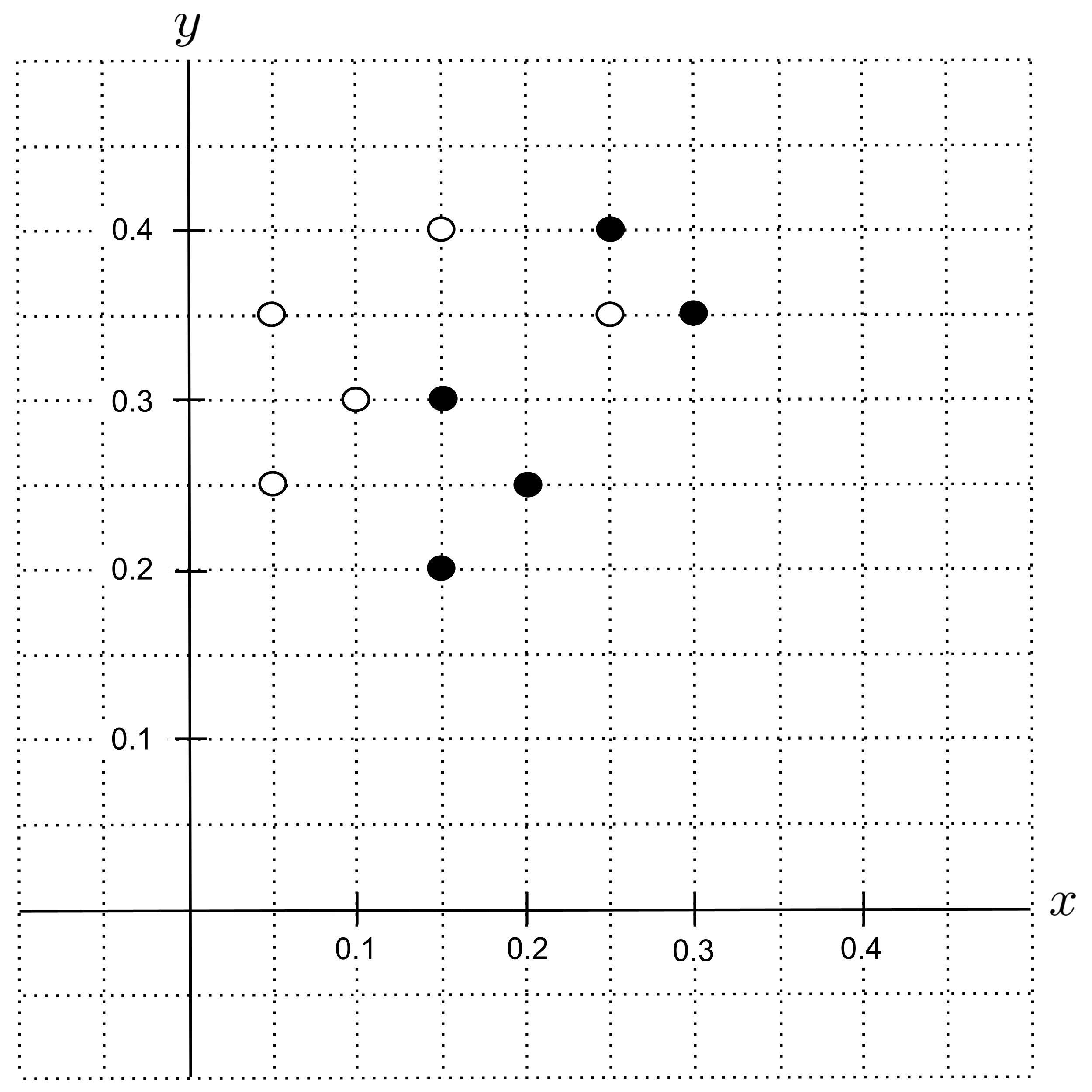
$\begin{align*} \begin{matrix} \textrm{Cookie Type} & \textrm{Portion Butter} & \textrm{Portion Sugar} \\ \hline \textrm{Shortbread} & 0.15 & 0.2 \\ \textrm{Shortbread} & 0.15 & 0.3 \\ \textrm{Shortbread} & 0.2 & 0.25 \\ \textrm{Shortbread} & 0.25 & 0.4 \\ \textrm{Shortbread} & 0.3 & 0.35 \\ \textrm{Sugar} & 0.05 & 0.25 \\ \textrm{Sugar} & 0.05 & 0.35 \\ \textrm{Sugar} & 0.1 & 0.3 \\ \textrm{Sugar} & 0.15 & 0.4 \\ \textrm{Sugar} & 0.25 & 0.35 \end{matrix} \end{align*}$

Let’s start by plotting the data. We’ll represent shortbread cookies using filled circles and sugar cookies using open circles. The $x$-axis will measure the portion butter, while the $y$-axis will measure the portion sugar.

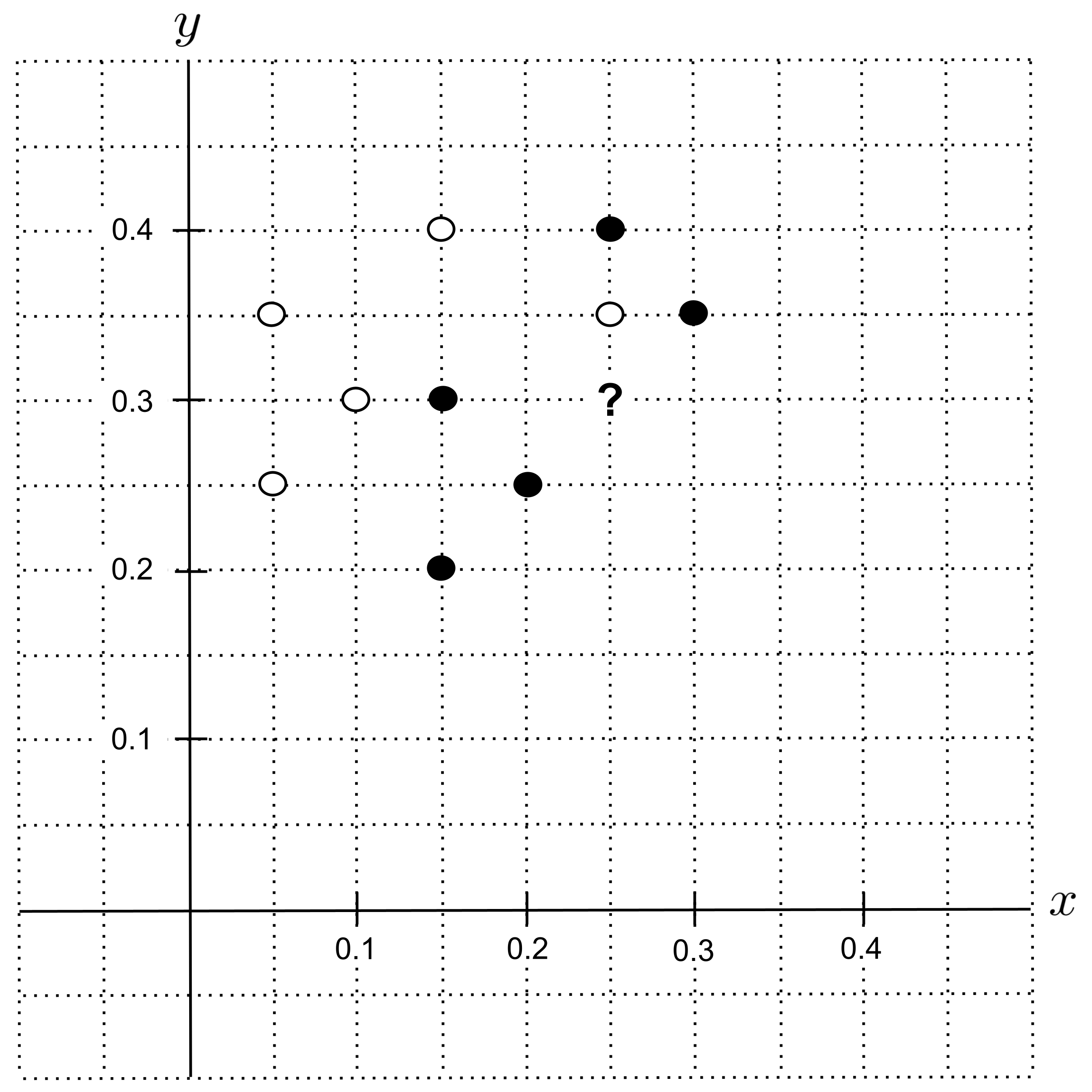
Suppose we have a cookie recipe that consists of $0.25$ portion butter and $0.3$ portion sugar, and we want to predict whether this is a shortbread cookie or a sugar cookie. First, we’ll identify the corresponding point $(0.25, 0.3)$ on our graph and label it with a question mark.

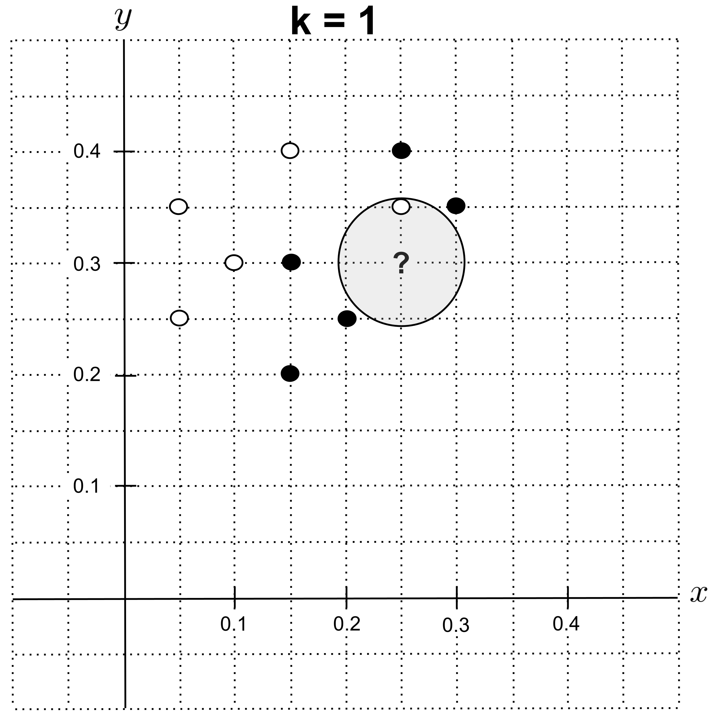
To identify the $k$ nearest neighbors of the unknown point, we can draw the smallest circle around the unknown point such that the circle contains $k$ other points from our data set.

The circle for $k=1$ is shown below. Since this nearest neighbor is a sugar cookie, we predict that the unknown cookie is also a sugar cookie.

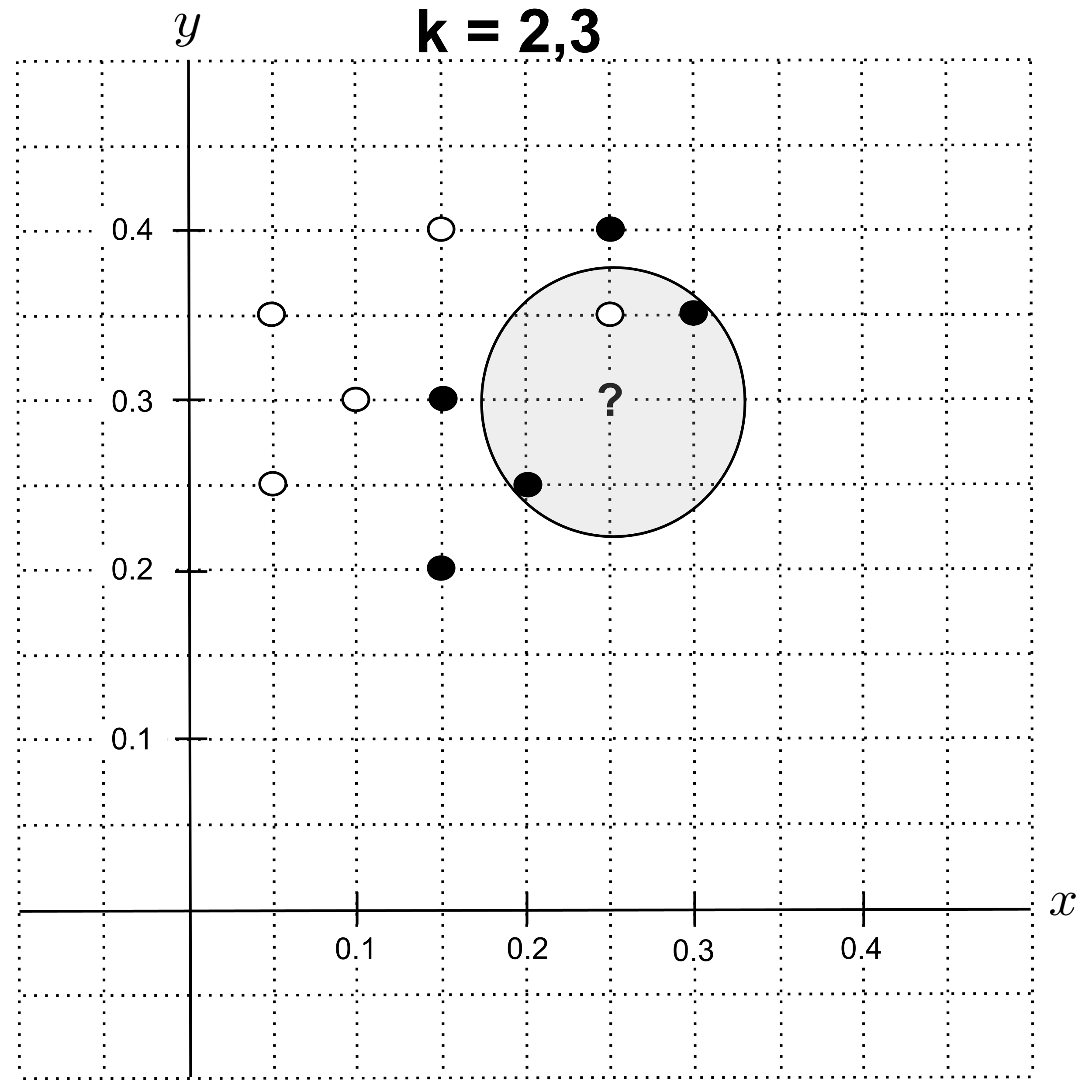
Using $k=2$ instead, we get the circle shown below. Notice that after the first nearest neighbor, the next two nearest neighbors are the same distance away from our unknown point, so we have to include both of them in our circle. Consequently, using $k=3$ gives us the exact same circle.

Now we have $3$ nearest neighbors: $2$ shortbread cookies and $1$ sugar cookie. As a result, the majority class is shorbtread, and we predict that the unknown cookie is a shortbread cookie.

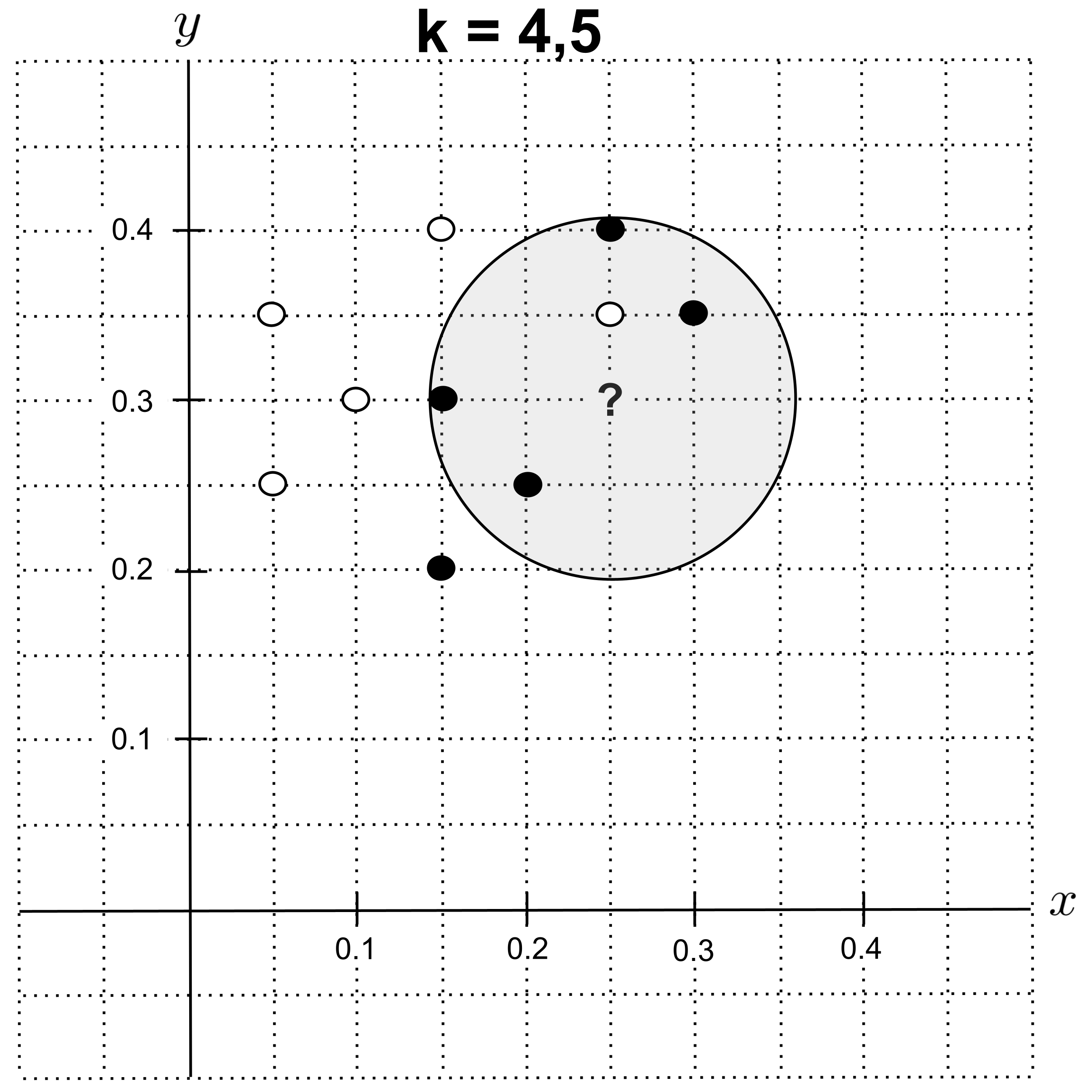
Using $k=4$ or $k=5,$ we get the circle below. The nearest neighbors are $4$ shortbread cookies and $1$ sugar cookie, so we predict that the unknown cookie is a shortbread cookie.

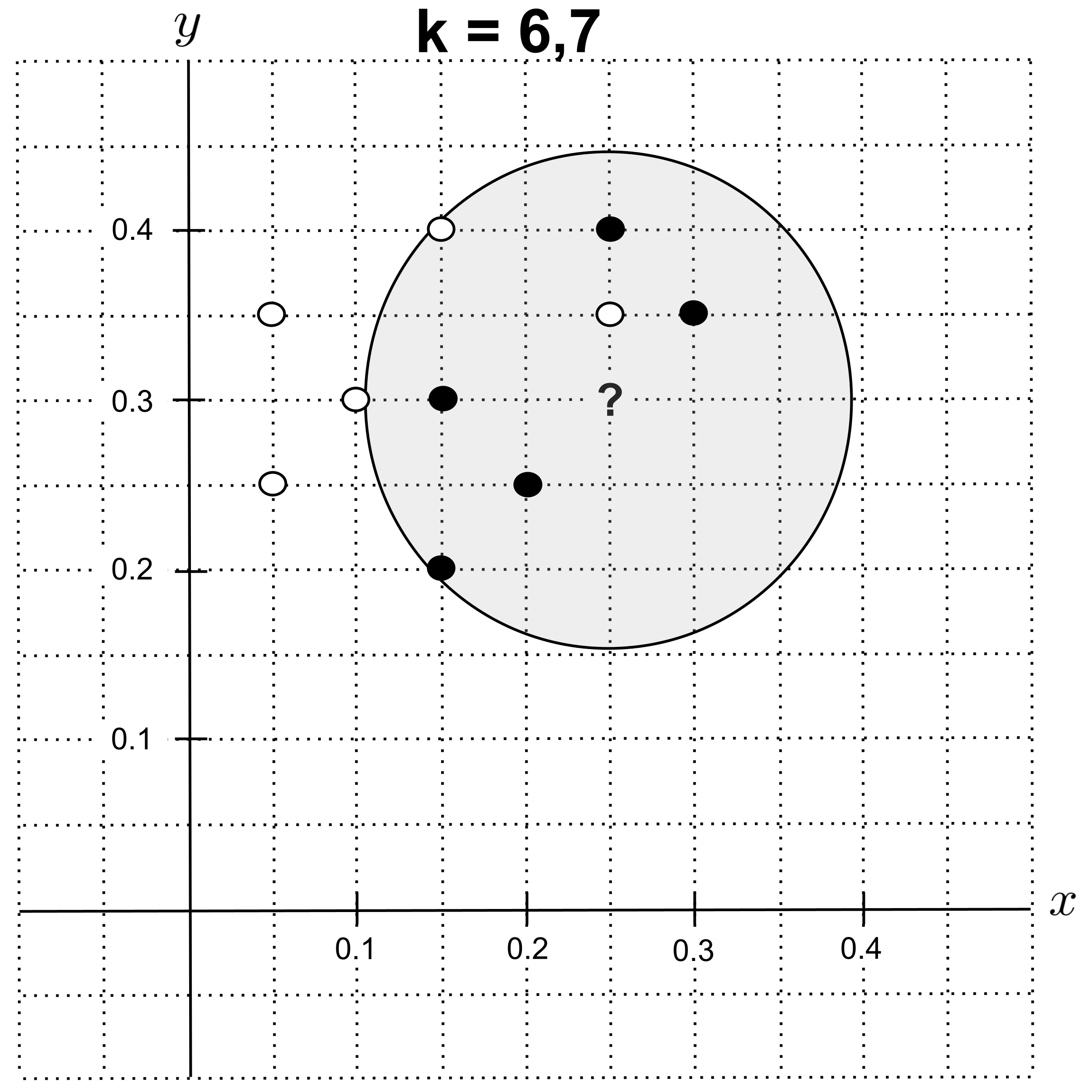
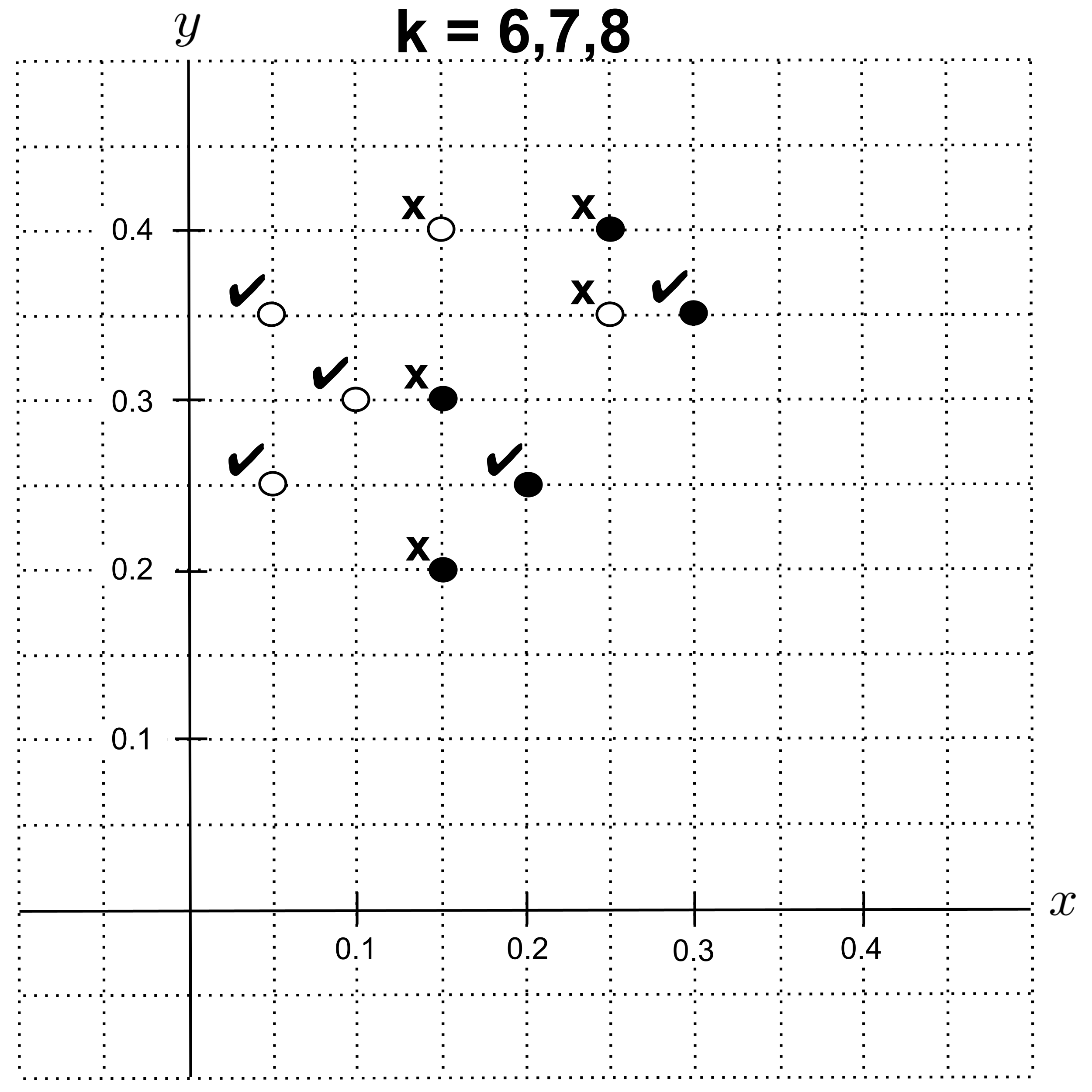
Using $k=6$ or $k=7,$ the nearest neighbors are $5$ shortbread cookies and $2$ sugar cookies, so we predict that the unknown cookie is a shortbread cookie.

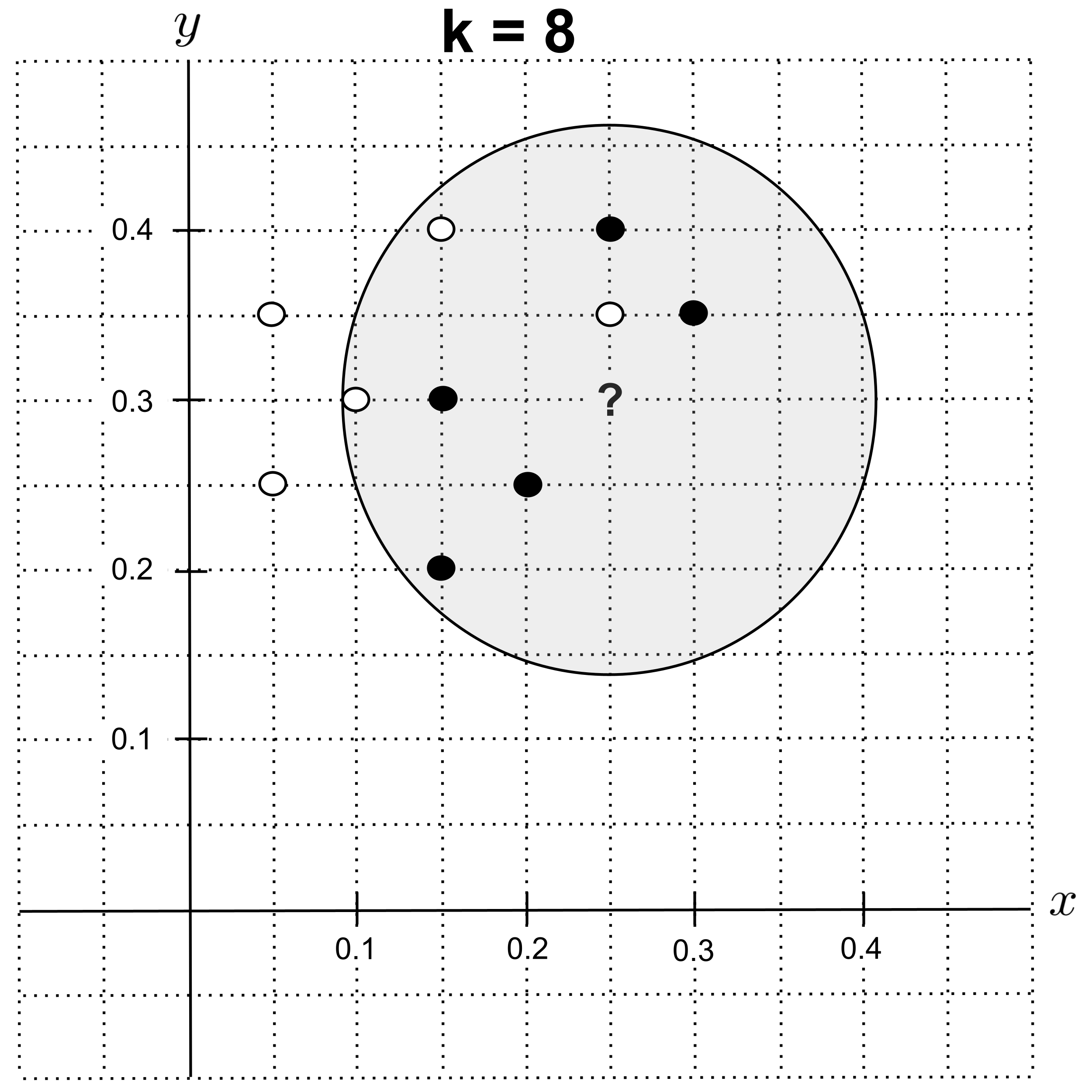
Using $k=8,$ the nearest neighbors are $5$ shortbread cookies and $3$ sugar cookies, so we predict that the unknown cookie is a shortbread cookie.

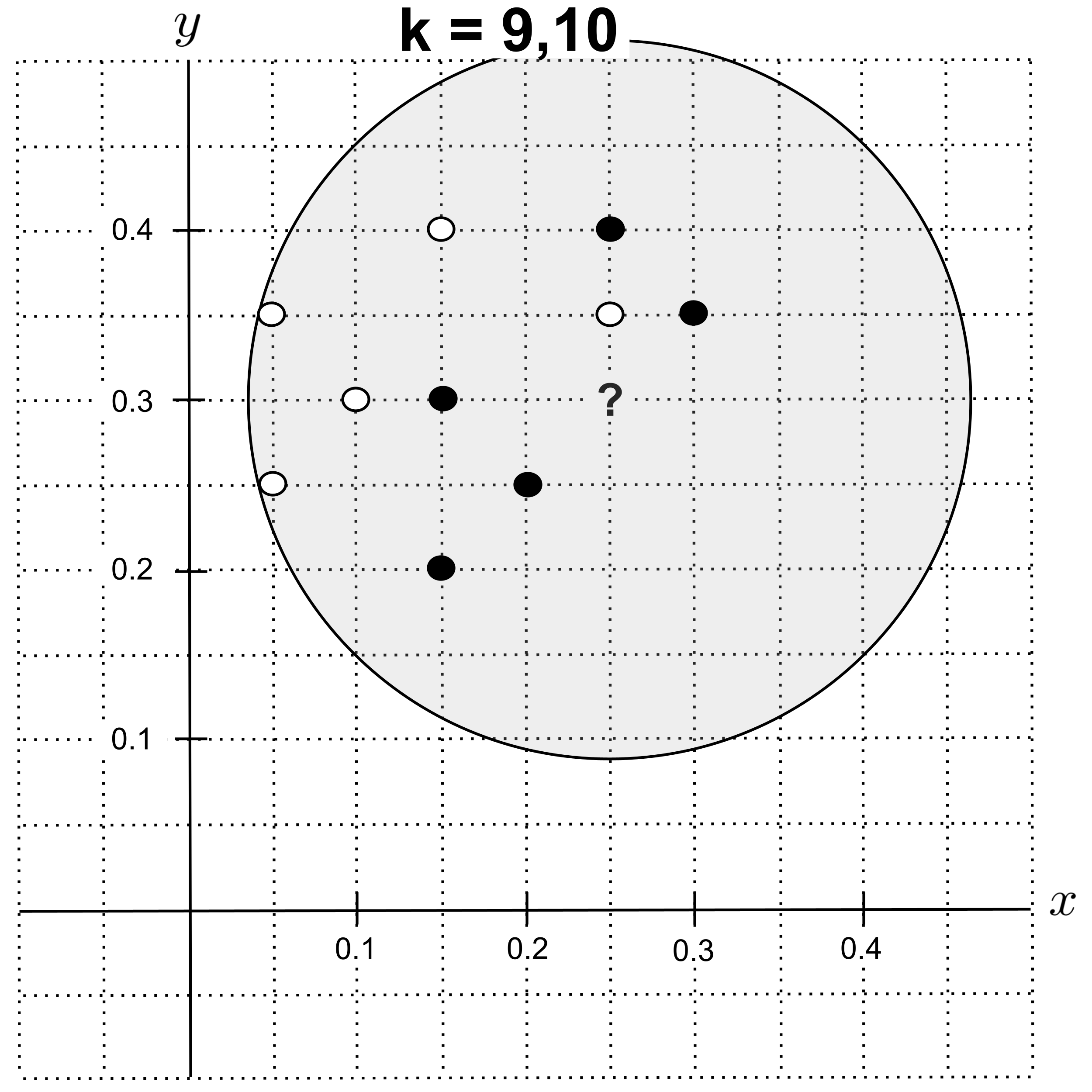
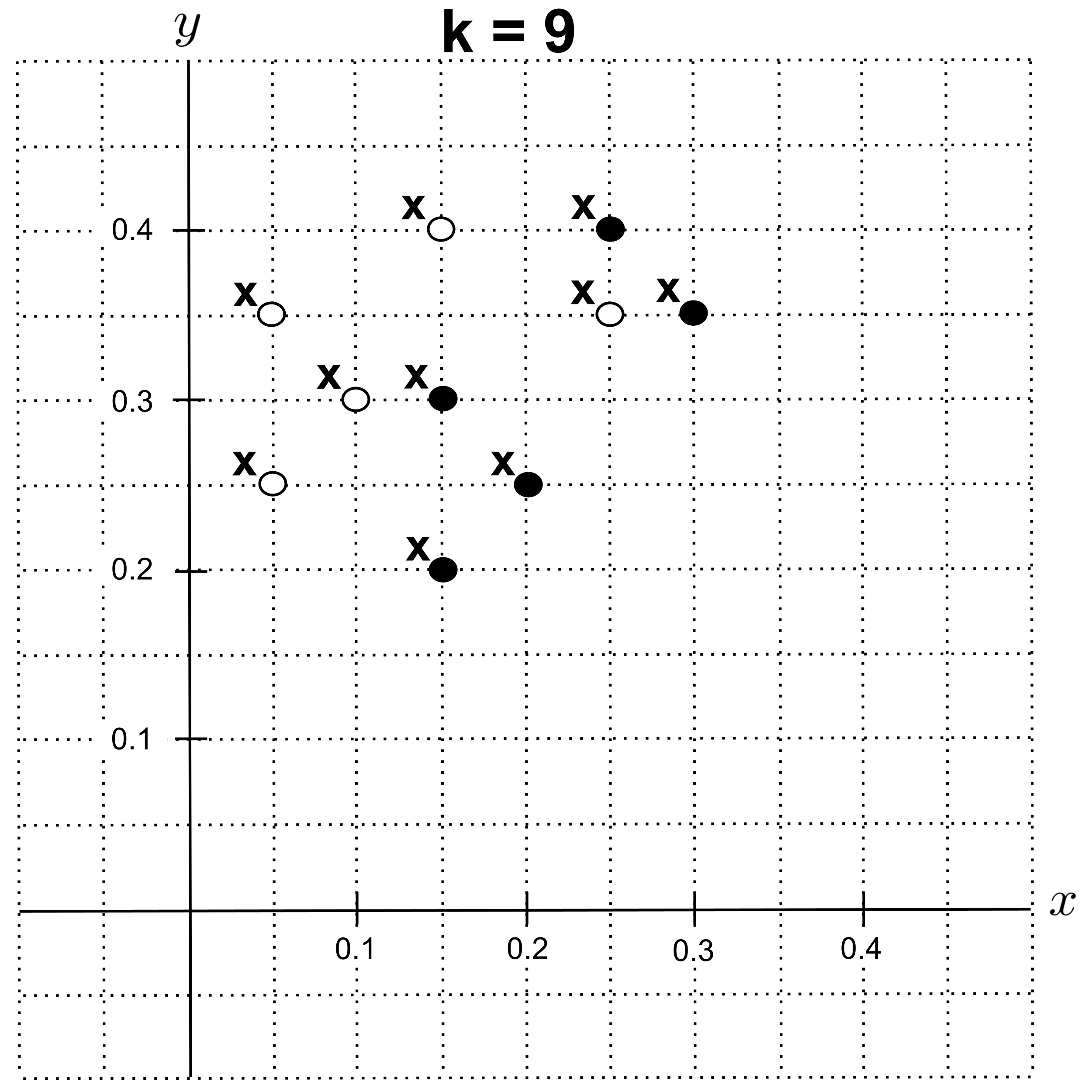
Using $k=9$ or $k=10,$ the nearest neighbors are $5$ shortbread cookies and $5$ sugar cookies. There is a tie for the majority class, so we will break the tie by choosing the class of nearest neighbors that has the lowest total distance from the unknown point.

We compute the distances of the nearest neighbors as follows:

$\begin{align*} \begin{matrix} \textrm{Cookie Type} & \textrm{Point} & \textrm{Distance From } (0.25,0.3) \\ \hline \textrm{Shortbread} & (0.15, 0.2) & \sqrt{(0.15-0.25)^2 + (0.2-0.3)^2}\phantom{00} &\approx 0.141 \\ \textrm{Shortbread} & (0.15, 0.3) & \sqrt{(0.15-0.25)^2 + (0.3-0.3)^2}\phantom{00} &= 0.1\phantom{00} \\ \textrm{Shortbread} & (0.2, 0.25) & \sqrt{(0.2-0.25)^2 + (0.25-0.3)^2}\phantom{00} &\approx 0.071 \\ \textrm{Shortbread} & (0.25, 0.4) & \sqrt{(0.25-0.25)^2 + (0.4-0.3)^2}\phantom{00} &= 0.1\phantom{00} \\ \textrm{Shortbread} & (0.3, 0.35) & \sqrt{(0.3-0.25)^2 + (0.35-0.3)^2}\phantom{00} &\approx 0.071 \\ \textrm{Sugar} & (0.05, 0.25) & \sqrt{(0.05-0.25)^2 + (0.25-0.3)^2}\phantom{0} &\approx 0.206 \\ \textrm{Sugar} & (0.05, 0.35) & \sqrt{(0.05-0.25)^2 + (0.35-0.3)^2}\phantom{0} &\approx 0.206 \\ \textrm{Sugar} & (0.1, 0.3) & \sqrt{(0.1-0.25)^2 + (0.3-0.3)^2}\phantom{000} &= 0.15\phantom{0} \\ \textrm{Sugar} & (0.15, 0.4) & \sqrt{(0.15-0.25)^2 + (0.4-0.3)^2}\phantom{00} &\approx 0.141 \\ \textrm{Sugar} & (0.25, 0.35) & \sqrt{(0.25-0.25)^2 + (0.35-0.3)^2}\phantom{0} &= 0.05\phantom{0} \end{matrix} \end{align*}$

Then, we compute the total distance for each class of nearest neighbors:

$\begin{align*} \textrm{Shortbread: } \,\,\, & 0.141 + 0.1\phantom{00} + 0.071 + 0.1\phantom{00} + 0.071 = 0.483 \\ \textrm{Sugar: } \,\,\, & 0.206 + 0.206 + 0.15\phantom{0} + 0.141 + 0.05\phantom{0} = 0.753 \end{align*}$

Since shortbread neighbors have a lower total distance from the unknown point, we predict that the unknown cookie is a shortbread cookie.

Choosing the Value of K

Now that we’ve learned how to make a prediction for any particular value of $k,$ the big question is: which value of $k$ should we use to make the prediction?

The value of $k$ is a parameter in k-nearest neighbors, just like the degree is a parameter in polynomial regression. To choose an appropriate degree for a polynomial regression, we used leave-one-out cross validation.

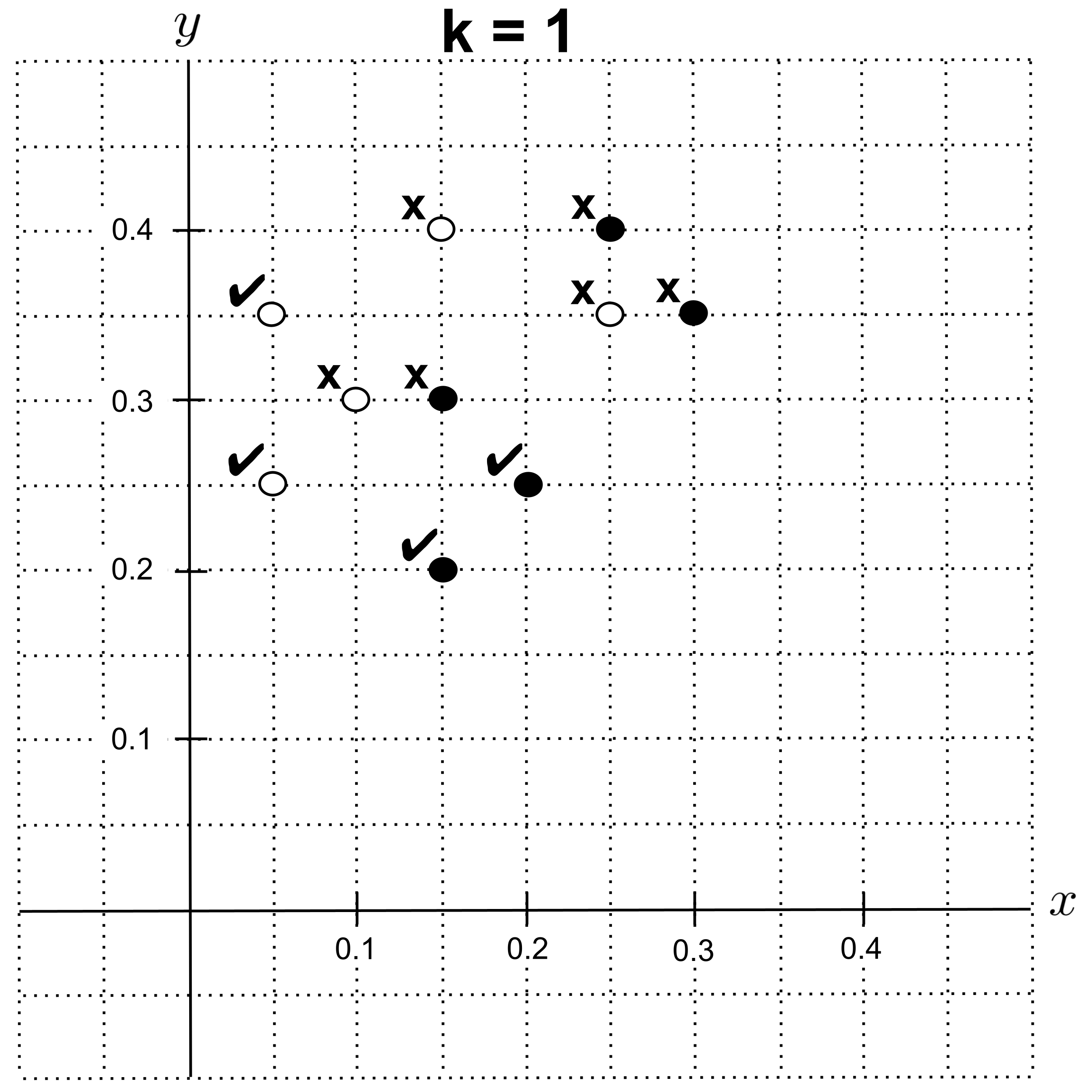
We can take the same approach here. The only difference is that instead of computing the residual sum of squares (RSS), we can directly compute the accuracy by dividing the number of correct classifications by the number of total classifications.

Using leave-one-out cross validation with $k=1,$ we get $4$ correct classifications out of $10$ total classifications, giving us an accuracy of $4 / 10 = 0.4.$

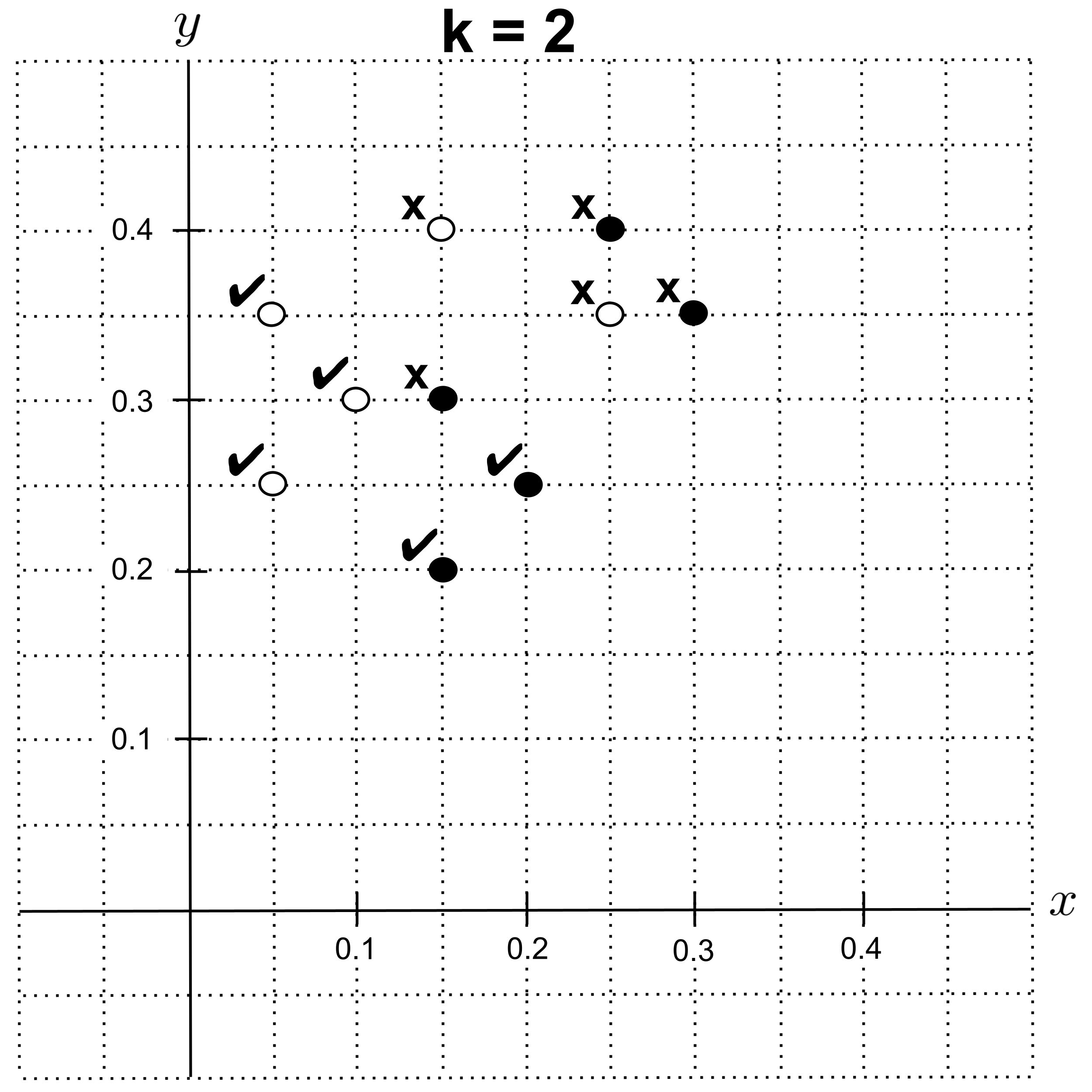
Using leave-one-out cross validation with $k=2,$ we get $5$ correct classifications, giving us an accuracy of $0.5.$

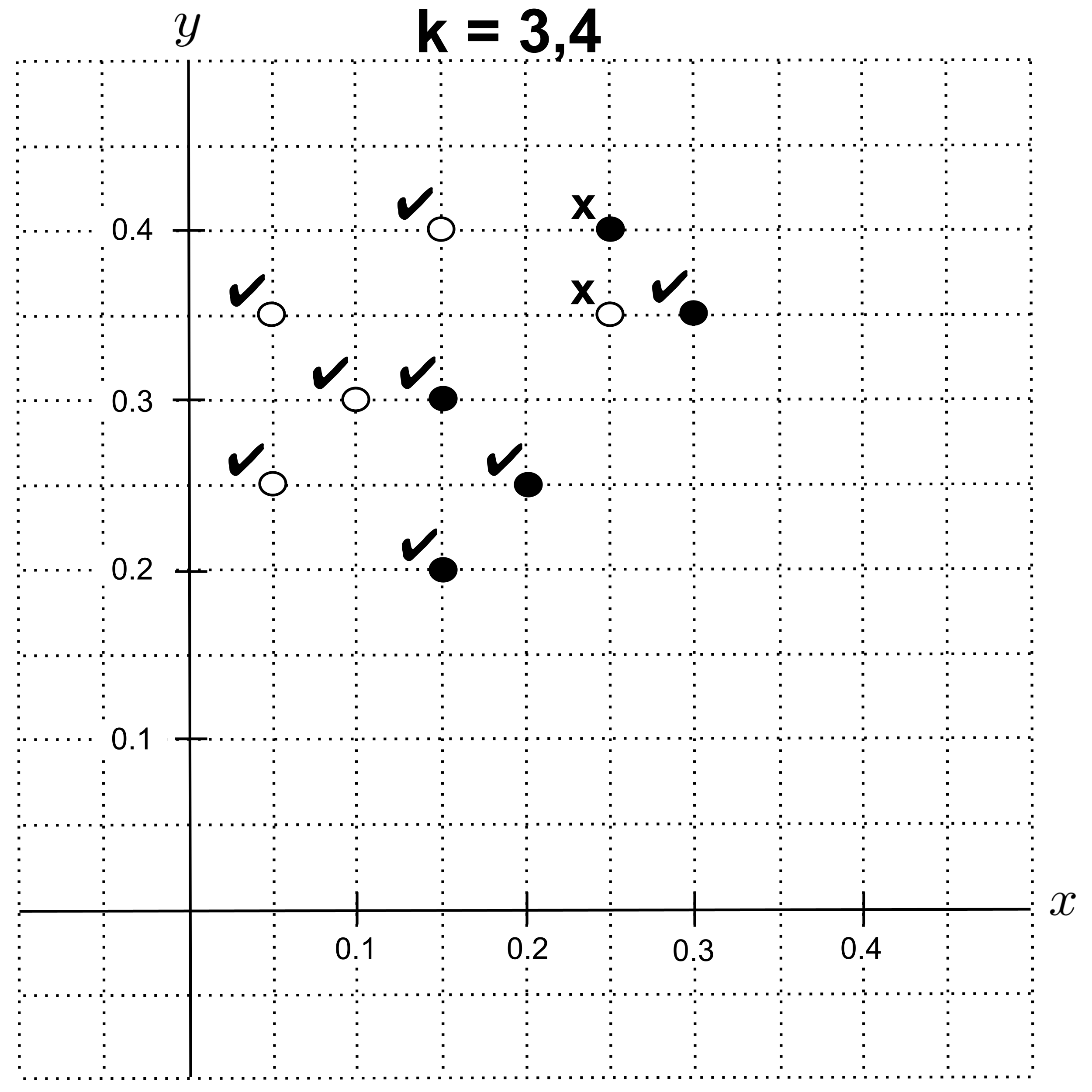
Using leave-one-out cross validation with $k=3$ or $k=4,$ we get an accuracy of $0.8.$

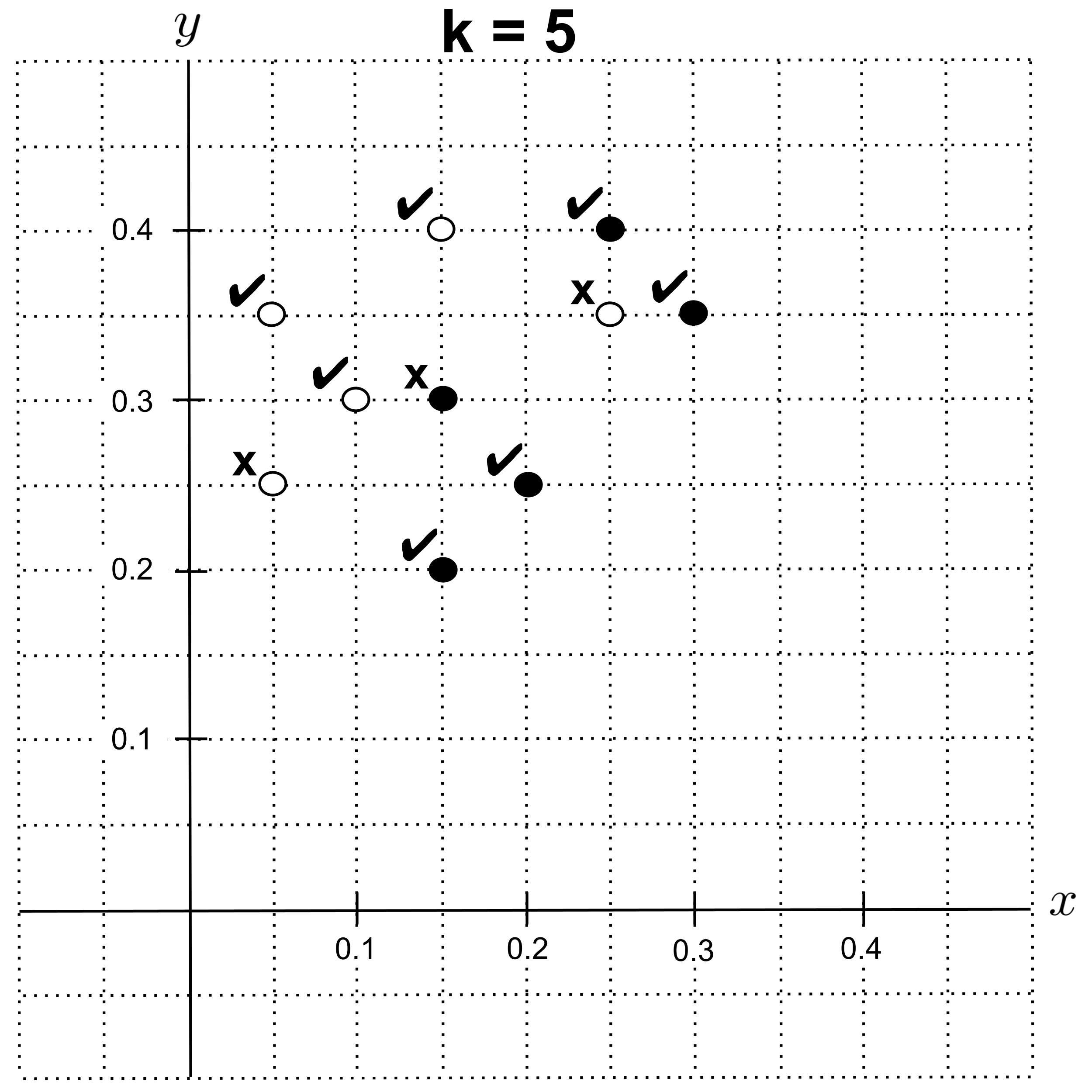
With $k=5,$ we get an accuracy of $0.7.$

With $k=6,$ $k=7,$ or $k=8,$ we get an accuracy of $0.5.$

With $k=9,$ we get an accuracy of $0.$ (Every point has $4$ nearest neighbors of the correct class and $5$ nearest neighbors of the incorrect class, leading us to predict the incorrect class.)

We organize our results in the graph below. The best fit (highest accuracy) occurred at $k=3$ and $k=4,$ so those would be good values of $k$ to use in our model.

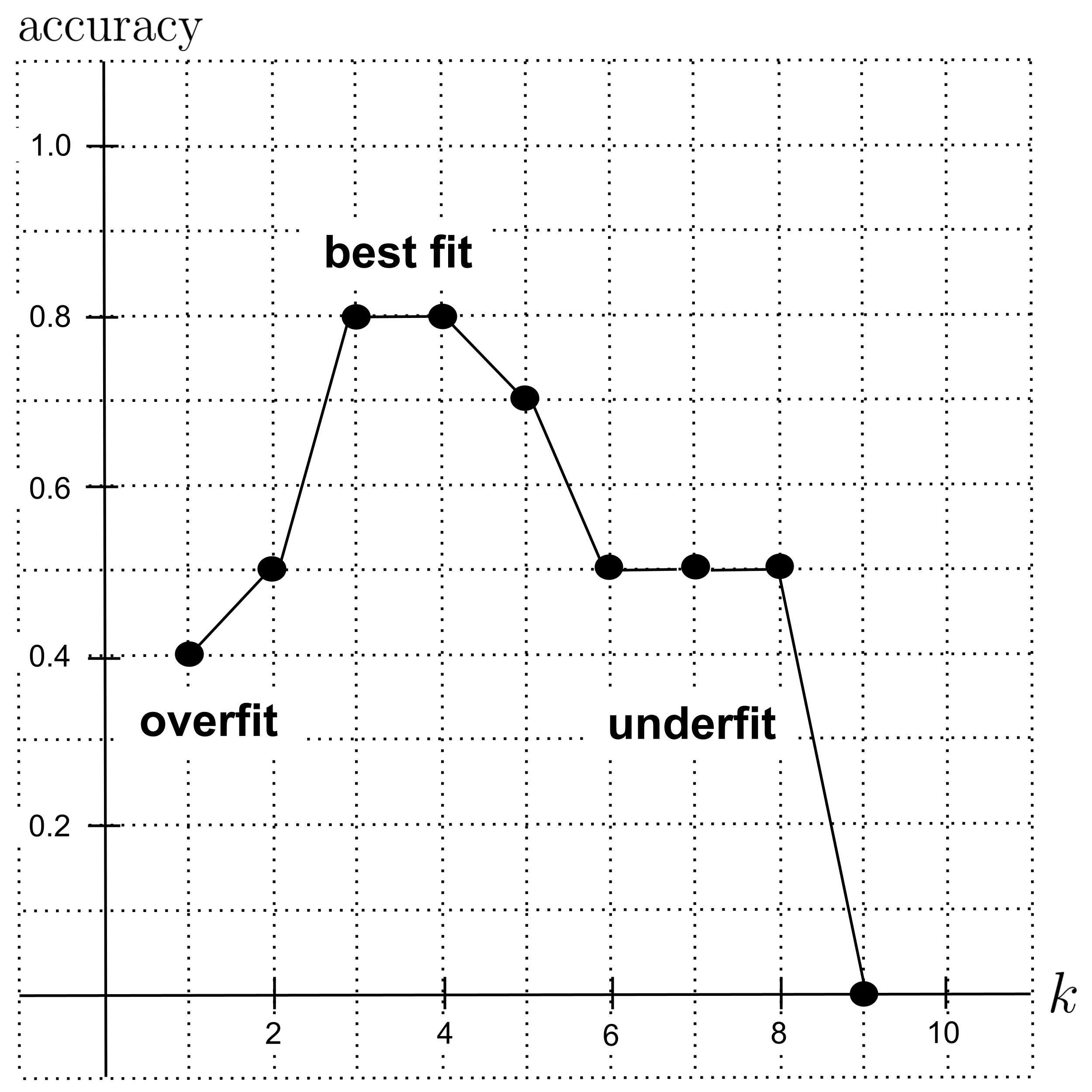
When $k$ is too low, the model overfits the data because it is too flexible (i.e. too high variance). In the extreme case of $k=1,$ the model only looks to a single nearest neighbor, which leads it to place too much trust in fine details (that could just be noise) instead of trying to understand the overall trend.

On the other hand, when $k$ is too high, the model underfits the data because it is too rigid (i.e. too high bias). In the extreme case where $k$ is equal to the number of points in the data set, the model totally ignores any sort of detail and will instead predict whichever class occurs most often in the data set.

In other words:

when $k$ is too low, the model relies too much on anecdotal evidence, and
when $k$ is too high, the model is unable to look beyond stereotypes.

Exercises

Implement the example that was worked out above. Start by classifying the unknown point $(0.25,0.3)$ for various values of $k,$ and then generate the leave-one-out cross validation curve.
Construct a cross-validation curve for the following data set, where we measure butter in cups and sugar in grams. The highest accuracy on this data set should be lower than the highest accuracy on the original data set. Why does using different scales for the variables cause worse performance? Run through the algorithm by hand until you notice and can describe what's happening.

$\begin{align*} \begin{matrix} \textrm{Cookie Type} & \textrm{Cups Butter} & \textrm{Grams Sugar} \\ \hline \textrm{Shortbread} & 0.6 & 200 \\ \textrm{Shortbread} & 0.6 & 300 \\ \textrm{Shortbread} & 0.8 & 250 \\ \textrm{Shortbread} & 1.0 & 400 \\ \textrm{Shortbread} & 1.2 & 350 \\ \textrm{Sugar} & 0.2 & 250 \\ \textrm{Sugar} & 0.2 & 350 \\ \textrm{Sugar} & 0.4 & 300 \\ \textrm{Sugar} & 0.6 & 400 \\ \textrm{Sugar} & 1.0 & 350 \end{matrix} \end{align*}$
As demonstrated by the previous problem, k-nearest neighbors models tend to perform worse when variables have different scales. To ensure that variables are measured on the same scale, it's common to normalize data before fitting models.

In particular, min-max normalization involves computing the minimum value of a variable, subtracting the minimum from all values, computing the new maximum value, and then dividing all values by that maximum. This ensures that the variable is measured on a scale from $0$ to $1.$

Normalize the "Cups Butter" variable in the data set above using min-max normalization. Then, do the same with the "Grams Sugar" variable. Finally, construct a cross-validation curve for the normalized data set and verify that the performance has improved.

Want to get notified about new posts? Join the mailing list and follow on X/Twitter.