K-Means Clustering

by Justin Skycak on March 03, 2021

Guess some initial clusters in the data, and then repeatedly update the guesses to make the clusters more cohesive.

This post is a chapter in the book Introduction to Algorithms and Machine Learning: from Sorting to Strategic Agents. Suggested citation: Skycak, J. (2021). K-Means Clustering. Introduction to Algorithms and Machine Learning: from Sorting to Strategic Agents. https://justinmath.com/k-means-clustering/

Clustering is the process of grouping similar records within data. Some examples of clusters in real-life data include users who buy similar items, songs in a similar genre, and patients with similar health conditions.

One of the simplest clustering methods is called k-means clustering. It works by guessing some initial clusters in the data and then repeatedly updating the guesses to make the clusters more cohesive.

Initialize the clusters.
1. Randomly divide the data into $k$ parts (where $k$ is an input parameter). Each part is an initial cluster.
2. Compute the mean of each part. Each mean is an initial cluster center.
Update the clusters.
1. Re-assign each record to the cluster with the nearest center.
2. Compute the new cluster centers by taking the mean of the records in each cluster.
Keep repeating step 2 until the clusters stop changing.

Worked Example

As a concrete example, consider the following data set. Each row represents a cookie with some ratio of ingredients. We can use k-means clustering to separate the data into different overarching “types” of cookies.


columns = ['Portion Eggs', 'Portion Butter', 'Portion Sugar', 'Portion Flour']

data = [
    [0.14, 0.14, 0.28, 0.44],
    [0.22, 0.1,  0.45, 0.33],
    [0.1,  0.19, 0.25, 0.4 ],
    [0.02, 0.08, 0.43, 0.45],
    [0.16, 0.08, 0.35, 0.3 ],
    [0.14, 0.17, 0.31, 0.38],
    [0.05, 0.14, 0.35, 0.5 ],
    [0.1,  0.21, 0.28, 0.44],
    [0.04, 0.08, 0.35, 0.47],
    [0.11, 0.13, 0.28, 0.45],
    [0.0,  0.07, 0.34, 0.65],
    [0.2,  0.05, 0.4,  0.37],
    [0.12, 0.15, 0.33, 0.45],
    [0.25, 0.1,  0.3,  0.35],
    [0.0,  0.1,  0.4,  0.5 ],
    [0.15, 0.2,  0.3,  0.37],
    [0.0,  0.13, 0.4,  0.49],
    [0.22, 0.07, 0.4,  0.38],
    [0.2,  0.18, 0.3,  0.4 ]
]

We will work out the first iteration of the k-means algorithm supposing that there are $k=3$ clusters in the data.

The first step is to randomly divide the data into $k=3$ clusters. To do this, we can simply add an extra column in our data that represents the cluster number, and count off cluster numbers $1,$ $2,$ $3,$ $1,$ $2,$ $3,$ and so on. We will put the extra column at the beginning of the data set.


[
    [1, 0.14, 0.14, 0.28, 0.44],
    [2, 0.22, 0.1,  0.45, 0.33],
    [3, 0.1,  0.19, 0.25, 0.4 ],
    [1, 0.02, 0.08, 0.43, 0.45],
    [2, 0.16, 0.08, 0.35, 0.3 ],
    [3, 0.14, 0.17, 0.31, 0.38],
    [1, 0.05, 0.14, 0.35, 0.5 ],
    [2, 0.1,  0.21, 0.28, 0.44],
    [3, 0.04, 0.08, 0.35, 0.47],
    [1, 0.11, 0.13, 0.28, 0.45],
    [2, 0.0,  0.07, 0.34, 0.65],
    [3, 0.2,  0.05, 0.4,  0.37],
    [1, 0.12, 0.15, 0.33, 0.45],
    [2, 0.25, 0.1,  0.3,  0.35],
    [3, 0.0,  0.1,  0.4,  0.5 ],
    [1, 0.15, 0.2,  0.3,  0.37],
    [2, 0.0,  0.13, 0.4,  0.49],
    [3, 0.22, 0.07, 0.4,  0.38],
    [1, 0.2,  0.18, 0.3,  0.4 ]
]

So, our initial guesses for the clusters are as follows:


# Cluster 1
[
    [1, 0.14, 0.14, 0.28, 0.44],
    [1, 0.02, 0.08, 0.43, 0.45],
    [1, 0.05, 0.14, 0.35, 0.5 ],
    [1, 0.11, 0.13, 0.28, 0.45],
    [1, 0.12, 0.15, 0.33, 0.45],
    [1, 0.15, 0.2,  0.3,  0.37],
    [1, 0.2,  0.18, 0.3,  0.4 ]
]

# Cluster 2
[
    [2, 0.22, 0.1,  0.45, 0.33],
    [2, 0.16, 0.08, 0.35, 0.3 ],
    [2, 0.1,  0.21, 0.28, 0.44],
    [2, 0.0,  0.07, 0.34, 0.65],
    [2, 0.25, 0.1,  0.3,  0.35],
    [2, 0.0,  0.13, 0.4,  0.49]
]

# Cluster 3
[
    [3, 0.1,  0.19, 0.25, 0.4 ],
    [3, 0.14, 0.17, 0.31, 0.38],
    [3, 0.04, 0.08, 0.35, 0.47],
    [3, 0.2,  0.05, 0.4,  0.37],
    [3, 0.0,  0.1,  0.4,  0.5 ],
    [3, 0.22, 0.07, 0.4,  0.38]
]

To compute each cluster center, we take the mean of each component of the data (ignoring the first component, which is the cluster label and was not part of the original data set).


# Cluster 1 center
[
    (0.14 + 0.02 + 0.05 + 0.11 + 0.12 + 0.15 + 0.2 ) / 7,
    (0.14 + 0.08 + 0.14 + 0.13 + 0.15 + 0.2  + 0.18) / 7,
    (0.28 + 0.43 + 0.35 + 0.28 + 0.33 + 0.3  + 0.3 ) / 7,
    (0.44 + 0.45 + 0.5  + 0.45 + 0.45 + 0.37 + 0.4 ) / 7
]

# Cluster 2 center
[
    (0.22 + 0.16 + 0.1  + 0.0  + 0.25 + 0.0 ) / 6,
    (0.1  + 0.08 + 0.21 + 0.07 + 0.1  + 0.13) / 6,
    (0.45 + 0.35 + 0.28 + 0.34 + 0.3  + 0.4 ) / 6,
    (0.33 + 0.3  + 0.44 + 0.65 + 0.35 + 0.49) / 6
]

# Cluster 3 center
[
    (0.1  + 0.14 + 0.04 + 0.2  + 0.0 + 0.22) / 6,
    (0.19 + 0.17 + 0.08 + 0.05 + 0.1 + 0.07) / 6,
    (0.25 + 0.31 + 0.35 + 0.4  + 0.4 + 0.4 ) / 6,
    (0.4  + 0.38 + 0.47 + 0.37 + 0.5 + 0.38) / 6
]

Carrying out the above computations, we get the following results (rounded to $3$ decimal places for readability):


# Cluster 1 center
[0.113, 0.146, 0.324, 0.437]

# Cluster 2 center
[0.122, 0.115, 0.353, 0.427]

# Cluster 3 center
[0.117, 0.110, 0.352, 0.417]

Once we’ve computed each cluster center, we then loop through the data and re-assign each data point to the nearest cluster center. We will use the Euclidean distance when determining the nearest cluster center.


Data point: [0.14, 0.14, 0.28, 0.44]
Distance
    from cluster 1 center: 0.052 <-- nearest
    from cluster 2 center: 0.080
    from cluster 3 center: 0.085

Data point: [0.22, 0.1, 0.45, 0.33]
Distance
    from cluster 1 center: 0.202
    from cluster 2 center: 0.169
    from cluster 3 center: 0.167 <-- nearest

Data point: [0.1, 0.19, 0.25, 0.4]
Distance
    from cluster 1 center: 0.095 <-- nearest
    from cluster 2 center: 0.132
    from cluster 3 center: 0.132

...

Data with re-assigned clusters:
[
    [1, 0.14, 0.14, 0.28, 0.44],
    [3, 0.22, 0.1,  0.45, 0.33],
    [1, 0.1,  0.19, 0.25, 0.4 ],
    ...
]

Interpreting the Clusters

If you repeat this process over and over, the cluster labels will eventually stop changing, indicating that every data point is assigned to the nearest cluster. In this example, it should be straightforward to interpret the meaning of your final clusters:

One cluster represents cookies with a greater proportion of sugar. These might be sugar cookies.
Another cluster represents cookies with a greater proportion of butter. These might be shortbread cookies.
Another cluster represents cookies with a greater proportion of eggs. These might be fortune cookies.

Elbow Method

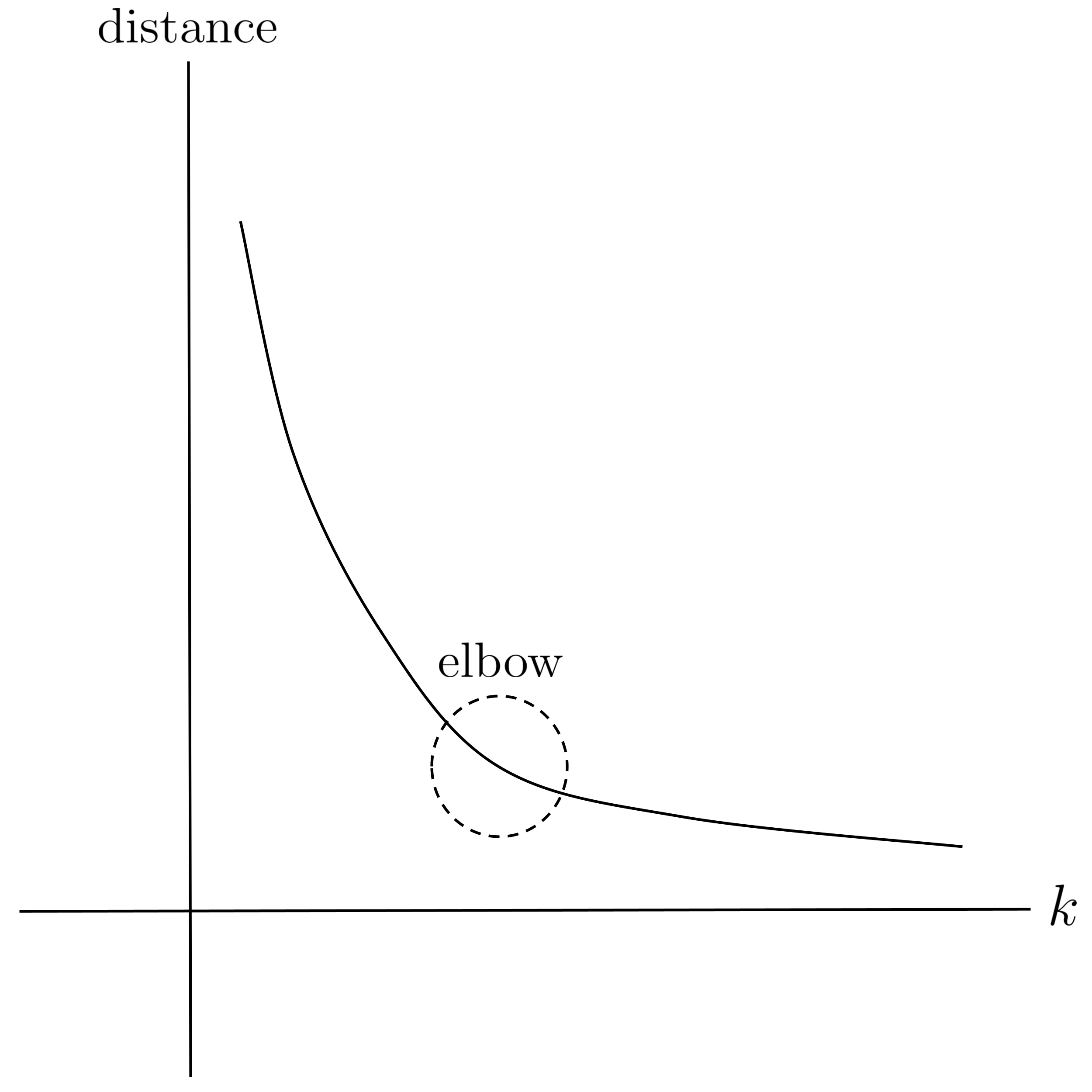
Finally, remember that $k$ (the number of clusters that we assume) is an input parameter to the algorithm. Because we usually don’t know the number of clusters in the data beforehand, it’s helpful to graph the “cohesiveness” of the clusters versus the value of $k.$ We can measure cohesiveness by computing the total sum of distances between points and their cluster centers (the smaller the total distance, the more cohesive the clusters).

The graph of total distance versus $k$ will be decreasing: the more clusters we assume, the closer the points will be to their clusters. In the extreme case where we set $k$ equal to the number of points in our data set, it’s possible that each point could be assigned to a separate cluster, resulting in a total distance of $0$ but providing us with absolutely no information about groups of similar records in the data.

To choose $k,$ it’s common to use the elbow method and roughly estimate where the graph forms an “elbow,” i.e. exhibits maximum curvature. This represents the point of diminishing returns, meaning that assuming a greater number of clusters in the data will not make the clusters that much more cohesive.

Exercises

First, implement the example that was worked out above and interpret the resulting clusters. Then, generate a plot of total distance versus $k$ and identify the elbow in the graph. Was $k=3$ a good choice for the number of clusters in our data set? In other words, is the elbow of the graph near $k=3?$