Intuiting Support Vector Machines
A Support Vector Machine (SVM) computes the "best" separation between classes as the maximum-margin hyperplane.
This post is part of the series Intuiting Predictive Algorithms.
Want to get notified about new posts? Join the mailing list and follow on X/Twitter.
In logistic regression, we maximize the likelihood of assigning the correct target class probability to a group of predictors. However, if our ultimate goal is to choose the most likely class for the group of predictors, we care less about getting the probability perfect when the choice of class is already determined (i.e. the probability is already fairly high or low), and more about choosing the correct class when the probability is borderline. In this case, we should focus on finding the best separation between the classes.
A Support Vector Machine (SVM) computes the “best” separation between classes as the maximum-margin hyperplane, i.e. the hyperplane that maximizes the distance of the closest points to the border (which are called the support vectors). For hyperplane of the form $w^Tx+b=0,$ we can assume $\vert \vert w \vert \vert=1$ because dividing the equation by $\vert \vert w \vert \vert$ yields the same plane, and thus the parameters $\theta = (w, b)$ that yield the maximum margin are given by
Through methods in constrained optimization, this “primal” form of the hyperplane can be reparametrized in “dual” form by the parameters $\alpha = (\alpha_i),$ one for each point in the data, which are chosen as
and for which the hyperplane is stated as
where the sum is taken over the support vectors.
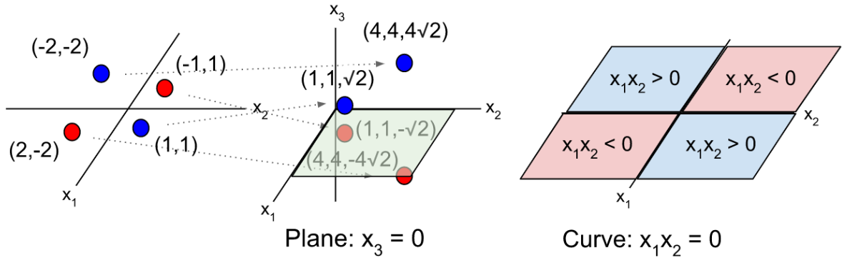
If the data is not linearly separable, then we can use a function $\phi: R^d \to R^{d+n}$ to map the data into a higher dimensional “feature” space before fitting the hyperplane. Below is an example of a function that maps 2-dimensional data $x_i = (x_{i1}, x_{i2})$ into 3-dimensional space.
The hyperplane, once projected to the lower-dimensional input space, is able to fit nonlinearities in the data.
Normally, we would worry about blowing up the number of dimensions in the model, which would cause computational and memory problems while training (fitting) the SVM. However, if we choose a function (like the one above) for that can be represented by a “kernel,” we can compute the result of dot products in the higher dimensional space, without having to compute and store the values of the data in the higher dimensional space:
This is called the “kernel trick.” Some common kernels include the homogeneous polynomial kernel $K(x_i,x_j) = (x_i^Tx_j)^d,$ the inhomogeneous polynomial kernel $K(x_i,x_j) = (x_i^Tx_j+1)^d,$ the Gaussian radial basis function (RBF) kernel $K(x_i,x_j) = \exp ( a x_i^Tx_j ),$ and the hyperbolic tangent kernel $K(x_i,x_j) = \tanh (ax_i^Tx_j + b).$
Another way to extend the SVM to data that is not linearly separable is to use a soft margin, where we minimize a loss function that penalizes data on the wrong side of the hyperplane. We introduce a “hinge loss” function that is zero for data on the correct side of the margin and is proportional to distance for data on the wrong side of the hyperplane, and minimize the total hinge loss:
The hinge loss function is named as such because its graph looks like a door hinge. When the data is linearly separable, the total hinge loss is minimized by our previous “hard margin” method. In practice, it is difficult to deal with the $||w||=1$ constraint, but we want to prevent the weights from blowing up, so we replace the constraint with a regularization:
A similar dual form exists for this minimization problem, on which the kernel trick is also applicable.
SVMs can be extended to multiclass problems by building a model for each pair of classes and then selecting the class that receives the most votes from the ensemble of models. This is called one-vs-one (OvO) classification.
Another option is to force the SVM to give a probabilistic score rather than binary output, build a model for each class against the rest of the data, and then select the class whose model gives the highest score. This is called one-vs-rest (OvR) classification. To induce a probabilistic score, one can interpret the distance from the hyperplane as the logit (log of the odds ratio) of the in-class probability:
SVMs can also be used for regression, in which case they are called Support Vector Regressors (SVRs). In SVRs, the support vectors are the furthest points from the hyperplane, and the task is to minimize the distance to the support vectors.
This post is part of the series Intuiting Predictive Algorithms.
Want to get notified about new posts? Join the mailing list and follow on X/Twitter.