Intuiting Adversarial Examples in Neural Networks via a Simple Computational Experiment

The network becomes book-smart in a particular area but not street-smart in general. The training procedure is like a series of exams on material within a tiny subject area (your data subspace). The network refines its knowledge in the subject area to maximize its performance on those exams, but it doesn't refine its knowledge outside that subject area. And that leaves it gullible to adversarial examples using inputs outside the subject area.

Background

Some years ago, I did a simple experiment on a neural network that really helped me understand why adversarial examples are possible.

The experiment involved training a fully-connected several-layer neural network (not convolutional) on the MNIST dataset of handwritten digits.

_________________________________________________________________
 Layer (type)                Output Shape              Param #   
=================================================================
 input (InputLayer)          [(None, 784)]             0         
                                                                 
 Layer_1 (Dense)             (None, 64)                50240     
                                                                 
 Layer_2 (Dense)             (None, 64)                4160      
                                                                 
 output (Dense)              (None, 10)                650       
                                                                 
=================================================================
Total params: 55,050
Trainable params: 55,050
Non-trainable params: 0
_________________________________________________________________

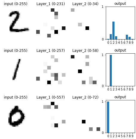
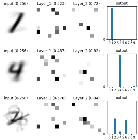
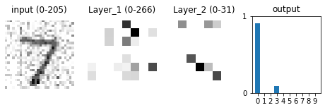
After training, I noticed that each input image activated only a small number of neurons in the network. For any given input image, there would be something like 3 highly-activated neurons, and 10 mildly-activated neurons, and the rest of the neurons would remain inactive. Each image’s representation within the network was distributed over a small number of neurons.

This led me to wonder what each neuron “does” in the network. Given any particular neuron, what does it detect? More precisely, what kind of features is it most attentive to in an input image?

Images that Maximally Activate Particular Neurons

Technically, the answer to this question is simple. To find the input image that maximally activates a neuron (i.e. the the input image that the neuron pays most attention to), all you have to do is look compute the neuron’s effective weight coming from each pixel in the input image.

• For a neuron in the first hidden layer, this is a simple lookup since it's connected directly to the input pixels.
• For a neuron in the second hidden layer, there are a handful of length-2 paths to any input pixel, and you just have to compute the product of the weights in each path and add up the results (though this can be phrased more elegantly as a weighted sum over the maximally-activating-images for the previous layer's neurons).

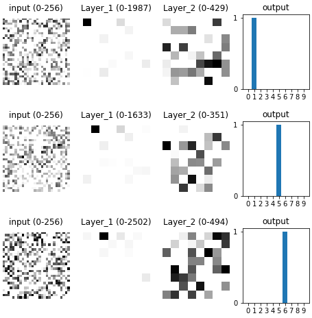
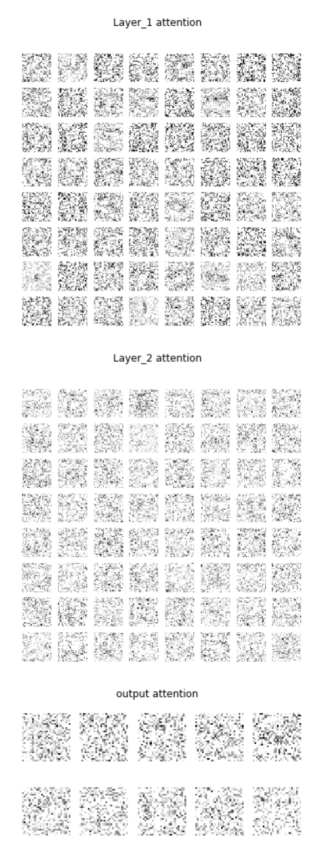
Below are the 3 images that maximally activate the first 3 neurons in the first hidden layer.

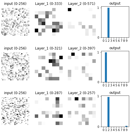
And the same for the first 3 neurons in the second hidden layer:

And the output layer:

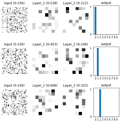
These results seemed kind of weird to me: the network was trained, and was classifying digits properly, and different neurons were paying more attention to different digits, as one might expect – but these neurons were still paying the most attention to images that looked like random noise.

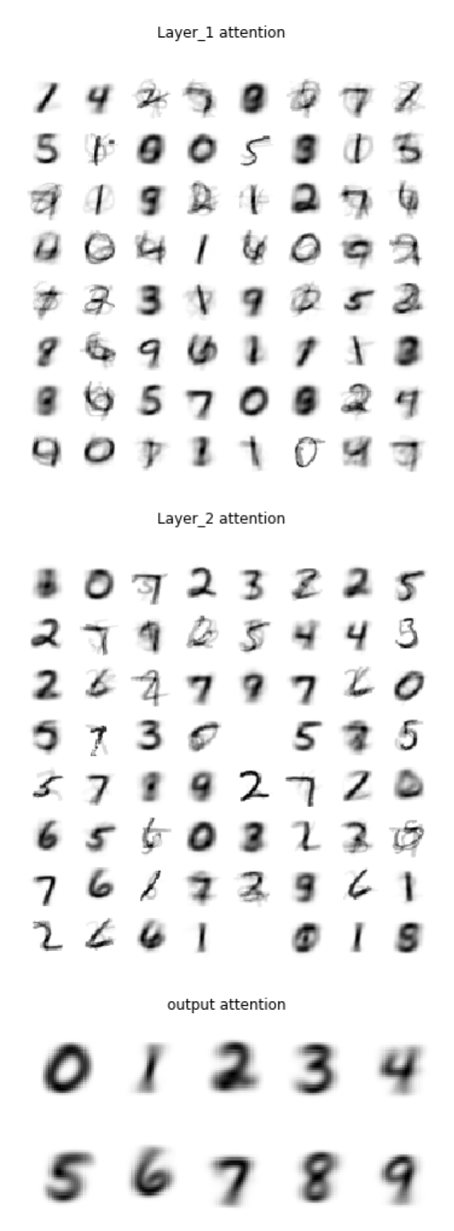
Limiting to Features Within the Dataset

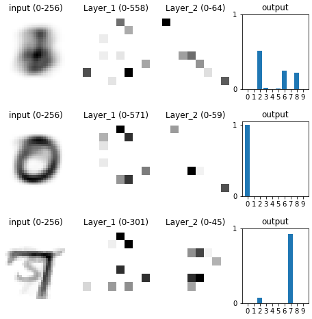
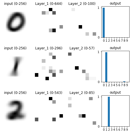
I began to suspect that there was a difference between what features a neuron pays most attention to overall versus within the dataset. Looking at the neuron’s input weights told us the former, not the latter. So, I revised my approach: to figure out what features a neuron was detecting within the dataset, I took a weighted average of all images in the dataset, weighted by the neuron’s activity in response to that input image.

Using this approach, I recreated the 4 diagrams from above. The results looked much more in line with what I was expecting.

And then it hit me what was really going on.

The Core Intuition

Of course, when you randomly initialize weights, the input image that maximally activates any particular neuron is going to look like randomly shaded pixels. And as you train the network on images in your data set, the network will adjust its weights as efficiently as possible to rectify its classifications of those images.

But the thing is, that only means the neuron has to become more discerning within the tiny subspace that your data occupies. The space of images in your dataset is a tiny subspace of all meaningful images, which is in turn a tiny subspace of all possible grids of shaded pixels. Even after the neuron adjusts its weights to be perfectly discerning within your data subspace, it probably hasn’t changed its opinion much about pixel grids outside that tiny subspace.

Basically, the network becomes book-smart in a particular area but not street-smart in general. The training procedure is like a series of exams on material within a tiny subject area (your data subspace). The network refines its knowledge in the subject area to maximize its performance on those exams, but it doesn’t refine its knowledge outside that subject area. And that leaves it gullible to adversarial examples using inputs outside the subject area.

For instance, if you take a digit 7 that your network classified correctly on the exam, and you overlay the random-looking pixel grid that maximally activates a neuron whose purpose is to detect the digit 0, then you can trick that neuron into believing (with extremely high confidence) that the digit in the image is 0, and thereby trick the entire network into thinking the same.