Hodgkin-Huxley Model of Action Potentials in Neurons

by Justin Skycak (@justinskycak) on March 07, 2021

Implementing a differential equations model that won the Nobel prize.

This post is part of the book Introduction to Algorithms and Machine Learning: from Sorting to Strategic Agents. Suggested citation: Skycak, J. (2021). Hodgkin-Huxley Model of Action Potentials in Neurons. In Introduction to Algorithms and Machine Learning: from Sorting to Strategic Agents. https://justinmath.com/hodgkin-huxley-model-of-action-potentials-in-neurons/

Want to get notified about new posts? Join the mailing list and follow on X/Twitter.

In 1952, Alan Hodgkin and Andrew Huxley published a differential equation model of “spikes” (i.e. “action potentials”) in the voltage of neurons. For this work, they received the 1963 Nobel Prize in Physiology or Medicine (shared with Sir John Carew Eccles).

Below, we summarize the key points of the model so that you may implement and simulate it yourself. The primary source is the original paper: A quantitative description of membrane current and its application to conduction and excitation in nerve.

For background information, it is recommended to watch the following short videos:

Neurons or nerve cells - Structure function and types of neurons by Elearnin
2-Minute Neuroscience: Action Potential by Neuroscientifically Challenged

Idea 1: Start with Physics Fundamentals

From physics, we know that current is proportional to voltage by a constant $C$ called the capacitance:

$\begin{align*} I = C \dfrac{\textrm dV}{\textrm dt} \end{align*}$

So, the voltage of a neuron can be modeled as

$\begin{align*} \dfrac{\textrm dV}{\textrm dt} = \dfrac{I}{C}. \end{align*}$

For neurons, we have $C \approx 1.0 \, .$

Idea 2: Decompose Current into Four Subcurrents (Stimulus and Ion Channels)

The current $I$ consists of

a stimulus $s$ to the neuron (from an electrode or other neurons),
current flux across sodium and potassium ion channels ($I_{\text{Na}}$ and $I_{\text K}$), and
current leakage, treated as a channel $I_{\text L}.$

The stimulus increases the voltage, while the flux and leakage decrease it. So, we have

$\begin{align*} \dfrac{\textrm dV}{\textrm dt} = \dfrac{1}{C} \left[ s - I_{\text{Na}} - I_{\text K} - I_{\text L} \right]. \end{align*}$

Idea 3: Model the Ion Channel Currents

The current across an ion channel is proportional to the voltage difference, relative to the equilibrium voltage of that channel:

$\begin{align*} I_{\text{Na}} (V,m,h) &= g_{\text{Na}}(m, h) \left( V - V_\text{Na} \right) &&V_\text{Na} \approx 115 \\[5pt] I_{\text{K}} (V,n) &= g_{\text{K}}(n) \left( V - V_\text{K} \right) &&V_{\text{K}\phantom{a}} \approx -12 \\[5pt] I_{\text{L}}(V) &= g_{\text{L}} \cdot \left( V - V_\text{L} \right) &&V_{\text{L}\phantom{a}} \approx 10.6 \end{align*}$

The constants of proportionality are conductances, which were modeled experimentally:

$\begin{align*} g_{\text{Na}}(m, h) &= \overline{g}_{\text{Na}} m^3 h &&\overline{g}_{\text{Na}} \approx 120 \\[5pt] g_{\text{K}}(n) &= \overline{g}_{\text{K}} n^4 &&\overline{g}_{\text{K}\phantom{a}} \approx 36 \\[5pt] g_{\text L} &= \overline{g}_\text{L} &&\overline{g}_{\text{L}\phantom{a}} \approx 0.3, \end{align*}$

where

$\begin{align*} \dfrac{\text dn}{\text dt} &= \alpha_n(V) (1-n) - \beta_n(V) n \\ \dfrac{\text dm}{\text dt} &= \alpha_m(V)(1-m) - \beta_m(V) m \\ \dfrac{\text dh}{\text dt} &= \alpha_h(V) (1-h) - \beta_h(V) h. \end{align*}$

and

$\begin{align*} \alpha_n(V) &= \dfrac{0.01(10-V)}{\exp \left[ 0.1 (10-V) \right] - 1} &&\beta_n(V) = 0.125 \exp \left[ -\dfrac{V}{80} \right] \\[5pt] \alpha_m(V) &= \dfrac{0.1(25-V)}{\exp \left[ 0.1 (25-V) \right] - 1} &&\beta_m(V) = 4 \exp \left[ - \dfrac{V}{18} \right] \\[5pt] \alpha_h(V) &= 0.07 \exp \left[ -\dfrac{V}{20} \right]&&\beta_{h\phantom{i}}(V) = \dfrac{1}{\exp \left[ 0.1( 30-V) \right] + 1}. \end{align*}$

Exercise

Your task is to implement the Hodgkin-Huxley neuron model using Euler estimation. You can represent the state of the neuron at time $t$ using

$\begin{align*} \Big( t, (V, n, m, h) \Big), \end{align*}$

and you can approximate the initial values by setting $V_0=0$ and setting $n,$ $m,$ and $h$ equal to their asymptotic values for $V_0=0{:}$

$\begin{align*} n_0 &= \dfrac{\alpha_n(V_0)}{\alpha_n(V_0) + \beta_n(V_0)} \\ m_0 &= \dfrac{\alpha_m(V_0)}{\alpha_m(V_0) + \beta_m(V_0)} \\ h_0 &= \dfrac{\alpha_h(V_0)}{\alpha_h(V_0) + \beta_h(V_0)} \end{align*}$

(When we take $V_0=0,$ we are letting $V$ represent the voltage offset from the usual resting potential.)

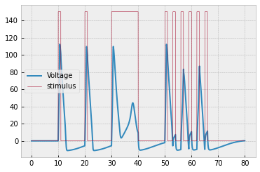
Simulate the system for $t \in [0, 80 \, \text{ms}]$ with step size $\Delta t = 0.01$ and stimulus

$\begin{align*} s(t) = \begin{cases} 150, & t \in [10,11] \cup [20,21] \cup [30,40] \cup [50,51] \cup [53,54] \\ & \phantom{t \in [} \cup [56,57] \cup [59,60] \cup [62,63] \cup [65,66] \\ 0 & \text{otherwise}. \end{cases} \end{align*}$

You should get the following result:

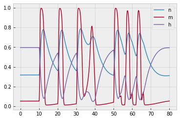
The corresponding plot of $n,$ $m,$ and $h$ is provided to help you debug:

Lastly, here is an incomplete code template to get you started:


###############################
### constants

V_0 = ...
n_0 = ...
m_0 = ...
h_0 = ...

C = 1.0
V_Na = 115
...

###############################
### main variables: V, n, m, h

def dV_dt(t,x):
	...

def dn_dt(t,x):
	n = x['n']
	return alpha_n(t,x) * (1-n) - beta_n(t,x) * n

def dm_dt(t,x):
	...

def dh_dt(t,x):
	...

###############################
### intermediate variables: alphas, betas, stimulus (s), currents (I's), ...

def alpha_n(t,x):
	...

def beta_n(t,x):
	...

...

################################
### input into EulerEstimator

derivatives = {
	'V': dV_dt,
	'n': dn_dt,
	...
}

initial_point = ...

Want to get notified about new posts? Join the mailing list and follow on X/Twitter.